Test of MQS + gauge

1. Introduction

In this page, I present the test case of Maxwell Quasi Static Problem in A-V Formulation with gauge condition for a geometry of torus surrounded by air for stationnary case.

2. Run the calculation

The command line to run this case is :

    mpirun -np 16 feelpp_toolbox_coefficientformpdes --config-file=magnetostatic.cfg --cfpdes.gmsh.hsize=5e-3

3. Data Files

The case data files are available in Github here :

CFG file - Edit the file
JSON file - Edit the file
GEO file - Edit the file

4. Equation

Thus \(\Omega\) the domain, comprising the conductor (or superconductor) domain \(\Omega_c\) and non conducting materials \(\Omega_n\) (\(\mathbf{J} = 0\)) like air. Let \(\Gamma = \partial \Omega\) the bound of \(\Omega\), \(\Gamma_c = \partial \Omega_c\) the bound of \(\Omega_c\), \(\Gamma_D\), \(\Gamma_{Dc}\) the bound with Dirichlet boundary condition and \(\Gamma_N\), \(\Gamma_{Nc}\) the bound with Neumann boundary condition, such that \(\Gamma = \Gamma_D \cup \Gamma_N\) and \(\Gamma_c = \Gamma_{Dc} \cup \Gamma_{Nc}\).

We introduce :

Magnetic potential field \(\mathbf{A}\) : the magnetic field writes \(\textbf{B} = \nabla \times \textbf{A}\)
Electric potential scalar : \(\nabla V = - \textbf{E}\)

We have the conditions :

\(\nabla \cdot \mathbf{A} = 0\)

We want to resolve the electromagnetism problem ( with \(\mathbf{A}\) and \(V\) the unknows) :

A-V Formulation with gauge condition

\[\text{(AV+gauge)} \left\{ \begin{matrix} \frac{1}{\mu} \Delta \textbf{A} &=& - \sigma \nabla V & \text{ on } \Omega & \text{(AV+gauge-1)} \\ \nabla \cdot \left( \sigma \nabla V \right) &=& 0 & \text{ on } \Omega_c & \text{(AV'-2)} \\ \mathbf{A} \times \mathbf{n} &=& 0 & \text{ on } \Gamma_D & \text{(DA)} \\ \left( \nabla \times \mathbf{A} \right) \times \mathbf{n} &=& 0 & \text{ on } \Gamma_N & \text{(NA)} \\ V &=& V_d & \text{ on } \Gamma_{Dc} & \text{(DV)} \\ \frac{\partial V}{\partial \mathbf{n}} &=& 0 & \text{ on } \Gamma_{Nc} & \text{(NV)} \end{matrix} \right.\]

This equation is obtain from the A-V Formulation with the gauge conditions. The detail calculus are in page MQS + gauge condition.

5. Geometry

The geometry is a quart of torus of conductor surrounded by air.

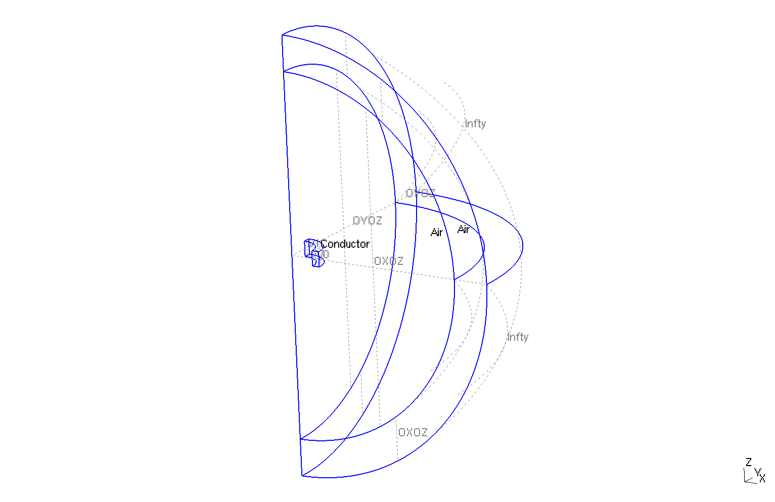
Geometry

The geometrical domains are :

Conductor (\(\Omega_c\)) : the torus, it is composed of conductive materials
- V0 : enter of electrical potential
- V1 : exit of electrical potential

(V0 \(\cup\) V1 \( = \Gamma_{Dc}\))

air (\(\Omega/\Omega_c\)) : the air surround Conductor
- OXOZ : \(OxOz\) plan
- OYOZ : \(OyOz\) plan
- Infty : the rest of bound of Air

Symbol

Description

value

unit

\(r_{int}\)

interior radius of torus

\(75e-3\)

\(r_{ext}\)

exterior radius of torus

\(100.2e-3\)

\(z_1\)

half-height of torus

\(25e-3\)

\(r_{infty}\)

radius of infty border

\(5*r_{ext}\)

6. Boundary Conditions

We impose the Dirichlet boundary conditions :

For \(V\) equation :
- On V0 : \(V=0\)
- On V1 : \(V = \frac{1}{4}\)
For \(\mathbf{A}\) :
- On OXOZ and V0 : \(A_x = A_z = 0\), we want \(\mathbf{A}\) orthogonal to OXOZ and V0
- On OYOZ and V1 : \(A_y = A_z = 0\), we want \(\mathbf{A}\) orthogonal to OYOZ and V1
- Infty : We approximate the problem, Infty is the physical infty thus \(\mathbf{B}=0\) at Infty thus \(\mathbf{A} = 0\).

We initialize at \(t=0s\) :

\(V = 0\)
\(\mathbf{A} = 0\)

On JSON file, the boundary conditions are writed :

Boundary conditions on JSON file

    "BoundaryConditions":
    {
        "magnetic":
        {
            "Dirichlet":
            {
                "Infty":
                {
                    "expr":"{0,0,0}"
                }
            },
            "Dirichlet_x":
            {
                "mydir_y":
                {
                    "markers":["V0","OXOZ"],
                    "expr":0
                }
            },
            "Dirichlet_y":
            {
                "mydir_y":
                {
                    "markers":["V1","OYOZ"],
                    "expr":0
                }
            },
            "Dirichlet_z":
            {
                "mydir_z":
                {
                    "markers":["V0","OXOZ","V1","OYOZ"],
                    "expr":0
                }
            }
        },
        "electric":
        {
            "Dirichlet":
            {
                "V0":
                {
                    "expr":"V0:V0"
                },
                "V1":
                {
                    "expr":"V1:V1"
                }
            }
        }
    }

7. Weak Formulation

The weak formulation of A-V Formulation + gauge is :

\[\text{(AV+gauge Weak)} \left\{ \begin{eqnarray*} \int_{\Omega}{ \frac{1}{\mu} \nabla \mathbf{A} \cdot \nabla \mathbf{ϕ} } &=& - \int_{\Omega_c}{\sigma \nabla V \, \mathbf{ϕ}} \\ \int_{\Omega_c}{ \sigma \nabla V \cdot \nabla \psi } &=& 0 \end{eqnarray*} \right.\]

8. Parameters

The parameters of problem are :

On Conductor :

Symbol

Description

Value

Unit

\(V0\)

scalar electrical potential on V0

\(0\)

\(Volt\)

\(V1\)

scalar electrical potential on V1

\(\frac{1}{4}\)

\(Volt\)

\(\sigma\)

electrical conductivity

\(58e6\)

\(S/m\)

\(\mu=\mu_0\)

magnetic permeability of vacuum

\(4\pi.10^{-7}\)

\(kg \, m / A^2 / S^2\)

On Air :

Symbol

Description

Value

Unit

\(\mu=\mu_0\)

magnetic permeability of vacuum

\(4\pi.10^{-7}\)

\(kg \, m / A^2 / S^2\)

On JSON file, the parameters are writed :

Parameters on JSON file

    "Parameters":
    {
        "V0":0,
        "V1":"1/4*(t/(0.1*10)*(t<(0.1*10))+((t<(0.5*40))+0*(t>(0.5*40)))*(t>(0.1*10))):t"
    }

9. Coefficient Form PDEs

We use the application Coefficient Form PDEs. The coefficient associate to Weak Formulation are :

In the json file, we note magnetic the equation (AV'-1) and electric the equation (AV'-2).

On Conductor :

Coefficient

Description

Expression

magnetic_c

diffusion coefficient

\(\frac{1}{\mu}\)

magnetic_f

source term

\(- \sigma \nabla V \)

electric_c

damping or mass coefficient

\(\sigma\)

On Air (the lectrical potential isn’t computed on Air) :

Coefficient

Description

Expression

magnetic_c

diffusion coefficient

\(\frac{1}{\mu}\)

On JSON file, the coefficients are writed :

CFPDEs coefficients on JSON file

    "Materials":
    {
        "Conductor":
        {
            "sigma":58e6,       // S.m-1
            "mu":"4*pi*1e-7",   // kg.m/A2/S2
            "magnetic_c":"1/mu:mu",
            "magnetic_f":"{-sigma*electric_grad_V_0,-sigma*electric_grad_V_1,-sigma*electric_grad_V_2}:sigma:electric_grad_V_0:electric_grad_V_1:electric_grad_V_2",

            "electric_c":"sigma:sigma"
        },
        "Air":
        {
            "physics":"magnetic",
            "mu":"4*pi*1e-7",   // kg.m/A2/S2
            "magnetic_c":"1/mu:mu"
        }
    }

10. Numeric Parameters

This section show the parameters used to compute the simulation.

Size of mesh :
- On Conductor : \(0.5 \, mm\)
- On Infty : \(100 \, mm\)
Element type : \(P1\)
Solver : automatic
Number of CPU core : \(16\)

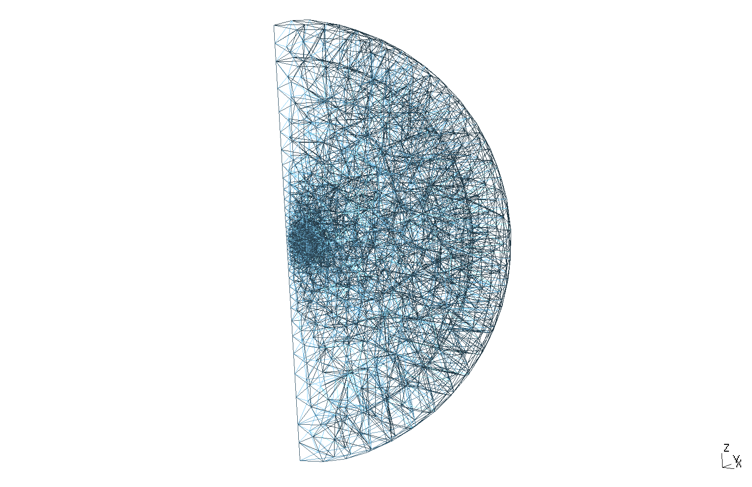
Mesh of Geometry

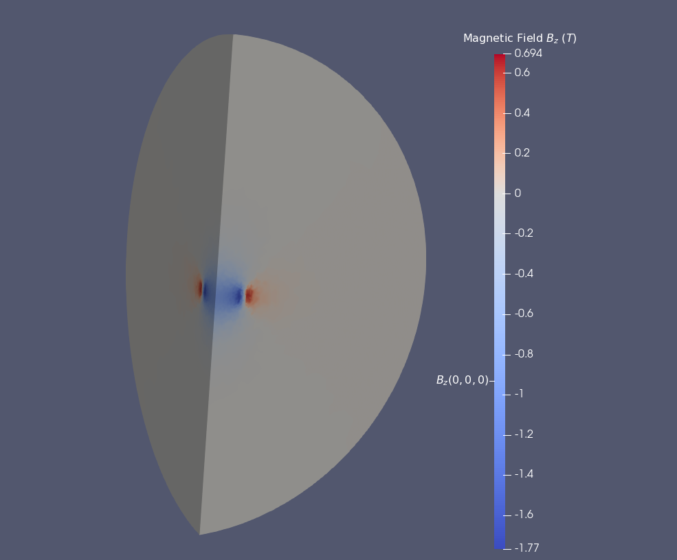
11. Result

11.1. Electric Potential Scalar \(V\)

We can see the value of electric potential scalar \(V\) on geometry :

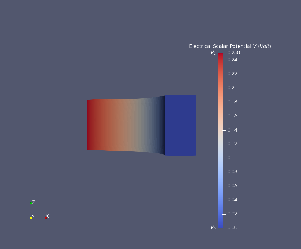
Components of \(V \, (Volt)\)

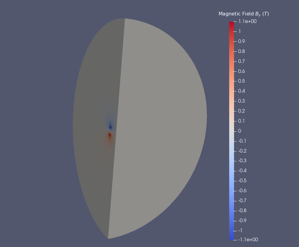
11.2. Potential Magnetic Field \(\mathbf{A}\)

I plot the the components of \(\mathbf{A}\) on \(O_r\) axis :

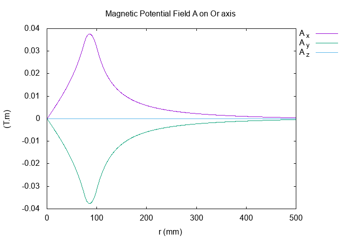
Components of \(\mathbf{A} \, (Tm)\) on Or axis

We can see the value of field on geometry :

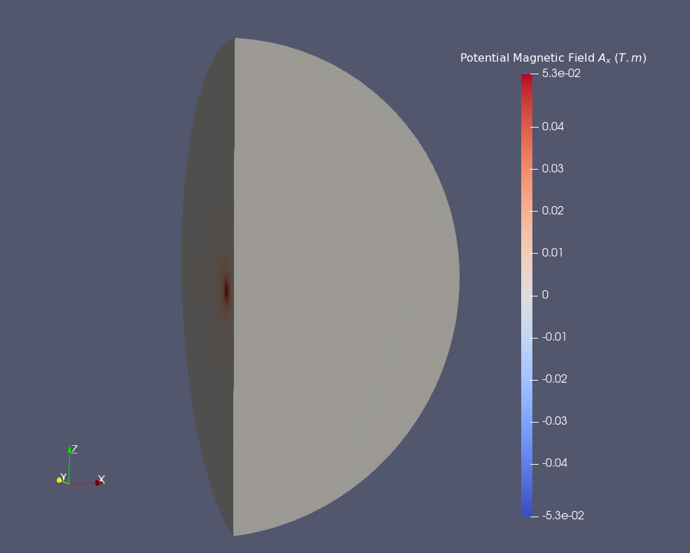
\(A_x \, (Tm)\) on Or axis

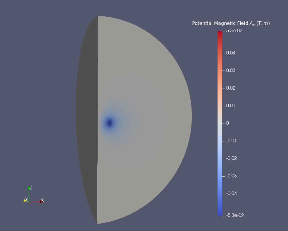
\(A_y \, (Tm)\) on Or axis

\(A_z \, (Tm)\) on Or axis

As predicted, the z component of potential magentic field \(A_z\) is equal to zeros.

11.3. Magnetic Field \(\mathbf{B}\)

I plot the the components of \(\mathbf{B}\) on a radius of tore :

Components of \(\mathbf{B} \, (T)\) on Or axis

We can see the value of field on geometry :

\(B_x \, (T)\) on Or axis

\(B_y \, (T)\) on Or axis

\(B_z \, (T)\) on Or axis

12. Validation

12.1. Exact solution

The analytical solve of potential magnetic field and magnetic field (the cyan curve on plots) is computed by python3’s module MagnetTools.MagnetTools. The module based on paper : spire. The python3’s script is here : Edit the file.

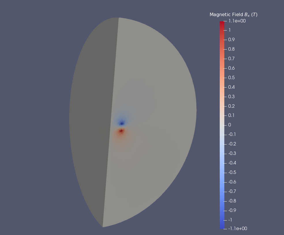
12.2. Convergence Test

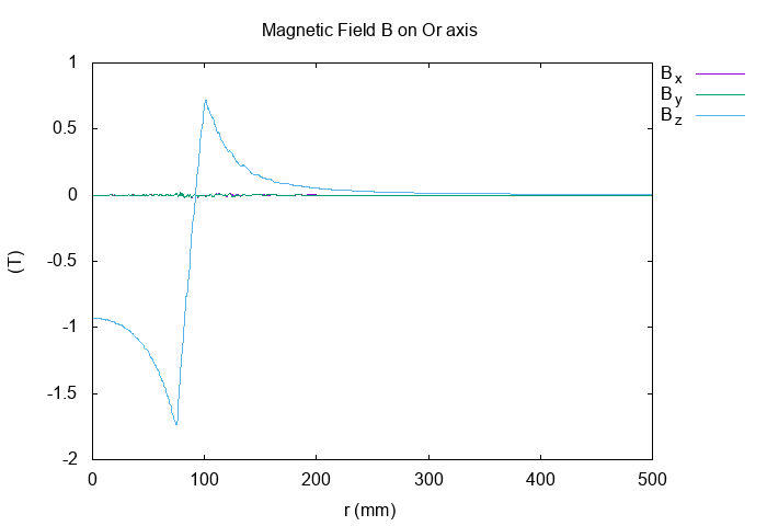
I plot the result of z component of magnetic field \(B_z\) on a radius of tore with exact solution computed with python3’s module MagnetTools.MagnetTools to "validate" the solution :

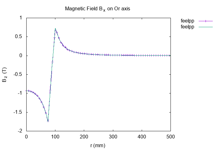
\(B_z (T)\) on Or axis

The two curves overlap, we have trust of our method.

We do the same for \(A_{\theta}\) (the orthoradial component in cylindrical coordinates) :

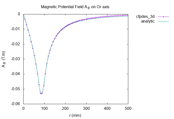
\(A_{\theta} (Tm)\) on Or axis

It exist a little difference near of Infty. To obtain better precision, we can increase the radius of Infty to have approximatively 0.

13. References

Calcul du champ magnétique pour les géométries axisymétriques simples, Christophe Trophime, 2002, unpublished, Download the PDF