Elastic Equations with Electromagnetism and Thermic in Axisymmetrical case

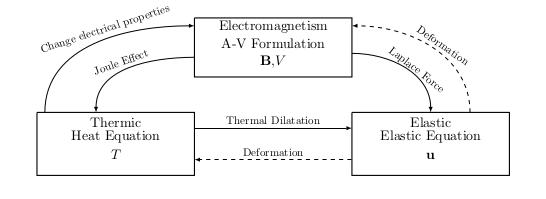
In page Elastic Equations in Electromagnetism and Thermic, we see the elastic equations with contribution of electromagnetism on displacement with Laplace Force and contribution of thermic with thermal dilatation. In this page, we rewrite those equations in axisymmetrical coordinates.

Diagram of Coupling problem

1. Recall

1.1. Axisymmetry

To define an axisymmetrical problem, we will place on cylindrical coordinates :

Set \(\left( x, \, y, \, z \right)\) the cartesian coordinates and \(\left( u_x, \, u_y, \, u_z \right)\) the cartesian basis. We write :

Cylindrical coordinates

\[\left\{ \begin{matrix} r = \sqrt{x^2+y^2} \\ \theta = arctan \left( \frac{y}{x} \right) \\ z =z \end{matrix} \right.\]

Cylindrical basis

\[\left\{ \begin{matrix} u_r = cos \theta \, u_x + sin \theta \, u_y \\ u_{\theta} = - sin \theta \, u_x + cos \theta \, u_y \\ u_z = u_z \end{matrix} \right.\]

We note \(u = \begin{pmatrix} u_r \\ u_{\theta} \\ u_z \end{pmatrix}_{cyl}\) the coordinates of \(u \in \mathbb{R}^3\) in cylindrical basis.

An axisymmetrical problem is a problem independant of of radial component (\(u_{\theta}\) and \(\theta\)). In the other words, an axisymmetrical problem is a problem symmetric by an axis, here \(Oz\). The problem can be geometrically describes with axisymmetrical coordinates \((r,z)\) and axisymmetrical basis \((u_r,u_z)\).

1.2. Thermo-magnetism model

This section retake the section Test Case in Axisymetric with Linear Coefficients.

We write the equations of coupled problem of Electromagnetism (in A-V Formulation) and Thermic.

Differential Formulation

\[\small{ \text{(AV-Heat)} \\ \left\{ \begin{matrix} \nabla \times \left( \frac{1}{\mu} \nabla \times \textbf{A} \right) + \sigma(T) \frac{\partial \textbf{A}}{\partial t} + \sigma(T) \nabla V &=& 0 & \text{ on } \Omega & \text{(AV-1)} \\ \nabla \cdot \left( \sigma(T) \nabla V + \sigma(T) \frac{\partial \textbf{A}}{\partial t} \right) &=& 0 & \text{ on } \Omega_c & \text{(AV-2)} \\ \rho C_p \, \frac{\partial T}{\partial t} - k(T) \Delta T &=& \sigma(T) \left( \nabla V + \frac{\partial \mathbf{A}}{\partial t} \right) \cdot \left( \nabla V + \frac{\partial \mathbf{A}}{\partial t} \right) & \text{ on } \Omega_c & \text{(Heat-1)} \\ \mathbf{A} \times \mathbf{n} &=& 0 & \text{ on } \Gamma_D & \text{(AV-D)} \\ \left( \nabla \times \mathbf{A} \right) \times \mathbf{n} &=& 0 & \text{ on } \Gamma_N & \text{(AV-N)} \\ \frac{\partial T}{\partial \mathbf{n}} &=& 0 & \text{ on } \Gamma_{Nc} & \text{(Heat-N)} \\ - k(T) \, \frac{\partial T}{\partial \mathbf{n}} &=& h \, \left( T - T_c \right) & \text{ on } \Gamma_{Rc} & \text{(Heat-R)} \\ \end{matrix} \right. }\]

With :

\(\mathbf{A}\) magnetic potential field

\(T\) temperature

\(V\) electrical potential scalar

\(k(T)=\frac{k_0}{1+\alpha (T-T_0)} \frac{T}{T_0}\) thermal conductivity

\(\sigma(T)=\frac{\sigma_0}{1+\alpha (T-T_0)}\) electrical conductivity

\(\rho\) density

\(C_p\) thermal capacity

\(T_c\) cooling temperature

\(T_0\) reference temperature

To pass in axisymmetrical coordinates, we suppose the variables, the temperature \(T\) and magnetic fields \(\mathbf{B} = \nabla \times \mathbf{A}\) are independant by \(\theta\) and the electric potential scalar \(V\) uniquely dependant by \(\theta\).

We note \(\Omega^{axis}\) (respectively \(\Omega^{axis}_c\), \(\Gamma^{axis}\), \(\Gamma_D^{axis}\), \(\Gamma_N^{axis}\), \(\Gamma_c^{axis}\), \(\Gamma_{Nc}^{axis}\) and \(\Gamma_{Rc}^{axis}\)) the representation of \(\Omega\) (respectively \(\Omega_c\), \(\Gamma\), \(\Gamma_D\), \(\Gamma_N\), \(\Gamma_c\), \(\Gamma_{Nc}\) and \(\Gamma_{Rc}\)) in axisymmetric coordinates.

We can rewrite the equations in axisymmetrical coordinates :

Differential Formulation in Axisymmetric

\[\text{(AV+Heat Axis)} \\ \left\{ \begin{matrix} \sigma \frac{\partial \Phi}{\partial t} - \frac{1}{\mu} \Delta \Phi + \frac{2}{\mu \, r} \frac{\partial \Phi}{\partial r} + \sigma \frac{\partial V}{\partial \theta} = 0 & \text{ on } \Omega^{axis} & \text{(AV-1 Axis)} \\ V = \frac{U}{2\pi} \, \theta & \text{ on } \Omega_c^{axis} & \text{(AV-2 Axis)} \\ A_{\theta} = 0 & \text{ on } \Gamma_D^{axis} & \text{(D Axis)} \\ \frac{\partial A_{\theta}}{\partial \mathbf{n}^{axis}} = 0 & \text{ on } \Gamma_N^{axis} & \text{(N Axis)} \\ \rho C_p \, \frac{\partial T}{\partial t} - k \Delta T = \sigma \, \left( \frac{1}{r} \, \frac{\partial V}{\partial \theta} + \frac{\partial A_{\theta}}{\partial t} \right)^2 & \text{ on } \Omega_c^{axis} & \text{(Heat Axis)} \\ \frac{\partial T}{\partial \mathbf{n}^{axis}} = 0 & \text{ on } \Gamma_{Nc}^{axis} & \text{(Nc Axis)} \\ - k \, \frac{\partial T}{\partial \mathbf{n}^{axis}} = h \, \left( T - T_c \right) & \text{ on } \Gamma_{Rc}^{axis} & \text{(Rc Axis)} \end{matrix} \right.\]

With \(\Phi = r \, A_{\theta}\)

1.3. Elastic Equations

This section retake the section Equation of Elasticity in Transient Case.

The elastic equations govern the displacement of conductor.

We introduce :

The displacemant \(\mathbf{u} = \begin{pmatrix} u_x \\ u_y \\ u_z \end{pmatrix}\)
The tensor of small deformation : \(\bar{\bar{\epsilon}} = \frac{1}{2} \left( \nabla \mathbf{u} + \nabla \mathbf{u}^T \right)\)
The stress tensor : \(\bar{\bar{\sigma}} = C(\bar{\bar{\epsilon}})\) with \(C\) a tensor which depends of the choice of elastic law.
The volumic Force : \(\mathbf{F}\)

Differential Formulation of Elasticity Equation

\[\text{(Elasticity)} \\ \left\{ \begin{matrix} \frac{\partial \mathbf{p}}{\partial t} - \nabla \cdot \bar{\bar{\sigma}} = \mathbf{F} & \text{on } \Omega_c & \text{(Elas-1)} \\ \mathbf{u} = \mathbf{u_0} & \text{on } \Gamma_{D \hspace{0.05cm} elas} & \text{(D elas)} \\ \bar{\bar{\sigma}} \cdot \mathbf{n} = g_N & \text{on } \Gamma_{N \hspace{0.05cm} elas} & \text{(N elas)} \\ \bar{\bar{\sigma}} \cdot \mathbf{n} + k \, \mathbf{u} = g_R & \text{on } \Gamma_{R \hspace{0.05cm} elas} & \text{(R elas)} \end{matrix} \right.\]

With :

Lamé’s coefficients : \(\lambda = \frac{E \, v}{(1-2 v) \, (1+v)}\), \(\mu = \frac{E}{2 \, (1+v)}\) with
- Young modulus \(E\)
- Poisson’s coefficient \(v\)
Displacement \(\mathbf{u} = \begin{pmatrix} u_x \\ u_y \\ u_z \end{pmatrix}\)
Momentum \(\mathbf{p} = \frac{\partial \left( \rho \, \mathbf{u} \right)}{\partial t} = \begin{pmatrix} p_x \\ p_y \\ p_z \end{pmatrix}\) with \(\rho\) the density
Stress Tensor : \(\bar{\bar{\sigma}}\)
Stiffness tensor : \(k\)
Volumic Force : \(\mathbf{F}\)

And notations :

Divergence of tensor : \(\nabla \cdot \bar{\bar{\sigma}} = \begin{pmatrix} \nabla \cdot \bar{\bar{\sigma}}_{x,:} \\ \nabla \cdot \bar{\bar{\sigma}}_{y,:} \\ \nabla \cdot \bar{\bar{\sigma}}_{z,:} \end{pmatrix} = \begin{pmatrix} \frac{\partial \bar{\bar{\sigma}}_{xx}}{\partial x} + \frac{\partial \bar{\bar{\sigma}}_{xy}}{\partial y} + \frac{\partial \bar{\bar{\sigma}}_{xz}}{\partial z} \\ \frac{\partial \bar{\bar{\sigma}}_{yx}}{\partial x} + \frac{\partial \bar{\bar{\sigma}}_{yy}}{\partial y} + \frac{\partial \bar{\bar{\sigma}}_{yz}}{\partial z} \\ \frac{\partial \bar{\bar{\sigma}}_{zx}}{\partial x} + \frac{\partial \bar{\bar{\sigma}}_{zy}}{\partial y} + \frac{\partial \bar{\bar{\sigma}}_{zz}}{\partial z} \end{pmatrix}\)
Scalar produce of tensor : \(\bar{\bar{\sigma}} \cdot \mathbf{n} = \begin{pmatrix} \bar{\bar{\sigma}}_{x,:} \cdot \mathbf{n} \\ \bar{\bar{\sigma}}_{y,:} \cdot \mathbf{n} \\ \bar{\bar{\sigma}}_{z,:} \cdot \mathbf{n} \end{pmatrix} = \begin{pmatrix} \bar{\bar{\sigma}}_{xx} \, n_x + \bar{\bar{\sigma}}_{xy} \, n_y + \bar{\bar{\sigma}}_{xz} \, n_z \\ \bar{\bar{\sigma}}_{yx} \, n_x + \bar{\bar{\sigma}}_{yy} \, n_y + \bar{\bar{\sigma}}_{yz} \, n_z \\ \bar{\bar{\sigma}}_{zx} \, n_x + \bar{\bar{\sigma}}_{zy} \, n_y + \bar{\bar{\sigma}}_{zz} \, n_z \end{pmatrix}\)

To pass in axisymmetrical coordinates, we suppose the variables and displacement \(\mathbf{B} = \nabla \times \mathbf{A}\) are independant by \(\theta\).

We note \(\Omega_c^{axis}\) (respectively \(\Gamma_c^{axis}\), \(\Gamma_{D \hspace{0.05cm} elas}^{axis}\), \(\Gamma_{N \hspace{0.05cm} elas}^{axis}\) and \(\Gamma_{R \hspace{0.05cm} elas}^{axis}\)) the representation of \(\Omega_c\) (respectively \(\Gamma_{D \hspace{0.05cm} elas}\), \(\Gamma_{N \hspace{0.05cm} elas}\) and \(\Gamma_{R \hspace{0.05cm} elas}\)) in axisymmetric coordinates.

We can rewrite the equations in axisymmetrical coordinates :

Differential Formulation of Elasticity Equation Case in Axisymmetric

\[\text{(Elasticity Axis)} \left\{ \begin{matrix} \frac{\partial \mathbf{p}}{\partial t} - \nabla \cdot \bar{\bar{\sigma}} = F & \text{on } \Omega_c^{axis} & \\ \mathbf{u} = 0 & \text{on } \Gamma_{D \hspace{0.05cm} elas}^{axis} & \text{(D axis elas)} \\ \bar{\bar{\sigma}} \cdot \mathbf{n}^{axis} = g_N & \text{on } \Gamma_{N \hspace{0.05cm} elas}^{axis} & \text{(N axis elas)} \\ \bar{\bar{\sigma}} \cdot \mathbf{n}^{axis} + k \, \mathbf{u} = g_R & \text{on } \Gamma_{R \hspace{0.05cm} elas}^{axis} & \text{(R axis elas)} \end{matrix} \right.\]

With : \(\mathbf{p} = \frac{\partial \left( \rho \, \mathbf{u} \right)}{\partial t}\) and \(\nabla \cdot \bar{\bar{\sigma}} = \begin{pmatrix} \nabla \cdot \bar{\bar{\sigma}}_{r,:} + \frac{\bar{\bar{\sigma}}_{rr} - \bar{\bar{\sigma}}_{\theta \theta}}{r} \\ \nabla \cdot \bar{\bar{\sigma}}_{z,:} + \frac{\bar{\bar{\sigma}}_{rz}}{r} \end{pmatrix}\)

2. Laplace Force

The Laplace Force is the macroscopic result of microscopic force Lorentz Force, and exprim like :

\[ \mathbf{F}_{laplace} = \mathbf{J} \times \mathbf{B}\]

With the current density \(\mathbf{J}\) and magnetic field \(\mathbf{B}\).

With equation \(\mathbf{J}=\sigma \, \mathbf{E}\) definition of magnetic potential field \(\mathbf{A}\) and electric potential scalar \(V\), we can rewrite :

\[ \mathbf{F}_{laplace} = \left( \sigma \, \left( - \nabla V - \frac{d \mathbf{A}}{d t} \right) \right) \times \left( \nabla \times \mathbf{A} \right)\]

We pass in axisymmetric coordinates :

\[\begin{eqnarray*} \mathbf{F}_{laplace} &=& - \sigma \left( \begin{pmatrix} 0 \\ \frac{1}{r} \frac{\partial V_{\theta}}{\partial \theta} \\ 0 \end{pmatrix}_{cyl} + \begin{pmatrix} 0 \\ \frac{d A_{\theta}}{d t} \\ 0 \end{pmatrix}_{cyl} \right) \times \begin{pmatrix} - \frac{\partial A_{\theta}}{\partial z} \\ 0 \\ \frac{1}{r} \frac{\partial \left( r A_{\theta} \right)}{\partial r} \end{pmatrix}_{cyl} \\ &=& - \sigma \begin{pmatrix} \left( \frac{1}{r} \frac{\partial V_{\theta}}{\partial \theta} + \frac{dA_{\theta}}{d t} \right) \ \frac{1}{r} \frac{\partial (r A_{\theta})}{\partial r} \\ 0 \\ \left( \frac{1}{r} \frac{\partial V_{\theta}}{\partial \theta} + \frac{dA_{\theta}}{d t} \right) \ \frac{\partial (A_{\theta})}{\partial z} \end{pmatrix}_{cyl} \\ &=& \begin{pmatrix} - \frac{\sigma}{r^2} \left( \frac{\partial V_{\theta}}{\partial \theta} + \frac{d \Phi}{dt} \right) \frac{\partial \Phi}{\partial r} \\ 0 \\ - \frac{\sigma}{r^2} \left( \frac{\partial V_{\theta}}{\partial \theta} + \frac{d \Phi}{dt} \right) \frac{\partial \Phi}{\partial z} \end{pmatrix}_{cyl} \end{eqnarray*}\]

Or, we can exprim like that :

\[\begin{eqnarray*] \mathbf{F}_{laplace} = \begin{pmatrix} \frac{1}{r} J_{\theta} \frac{\partial \Phi}{\partial r} \\ \frac{1}{r} J_{\theta} \frac{\partial \Phi}{\partial z} \end{pmatrix}_{cyl} \end{eqnarray*}\]

3. Thermal Dilatation

The temperature is the physic phenomena of micro movements of atoms of matters. The higher the temperature, the more the atoms take up space and the matter expands.

To modelize this thermal dilatation, we add a dilatation term to stress tensor Hook’s law :

\[ \bar{\bar{\sigma}}(\bar{\bar{\epsilon}}) = \bar{\bar{\sigma}}^E(\bar{\bar{\epsilon}}) + \bar{\bar{\sigma}}^T(\bar{\bar{\epsilon}})\]

With :

term of Hook’s law : \(\bar{\bar{\sigma}}^E(\bar{\bar{\epsilon}}) = \lambda \, Tr(\bar{\bar{\epsilon}}) + 2\mu \bar{\bar{\epsilon}}\)
dilatation term : \(\bar{\bar{\sigma}}^T(\bar{\bar{\epsilon}}) = - \frac{E}{1-2\xi} \, \alpha_T \, \left( T - T_0 \right) \, Id\), with linear dilatation coefficient \(\alpha_T\) and the reference temperature \(T_0\)

With formula of axisymmetric passage (with matrix of passage to cartesian to cylindric \(\small{P=\begin{pmatrix} cos\theta && sin\theta && 0 \\ -sin\theta && cos\theta && 0 \\ 0 && 0 && 1 \end{pmatrix}}\)) :

\[\begin{eqnarray*} \bar{\bar{\sigma}}^T(\bar{\bar{\epsilon}}) &=& P \, \left( - \frac{E}{1-2\xi} \, \alpha_T \, \left( T - T_0 \right) \, Id \right) \, P^{-1} \\ &=& - \frac{E}{1-2\xi} \, \alpha_T \, \left( T - T_0 \right) \, Id \end{eqnarray*}\]

We pass to axisymmetrical coordinates :

4. Elastic Thermic Electromagnetism model

4.1. Differential Formulation

The coupled equation of Elastic equations, Heat equation and A-V Formulation :

Differential Formulation of Elastic Thermic Electromagnetism equation in Axisymmetric

\[\text{(Elasto-Thermo-Elec Axis)} \\ \left\{ \begin{matrix} \sigma \frac{\partial \Phi}{\partial t} - \frac{1}{\mu} \Delta \Phi + \frac{2}{\mu \, r} \frac{\partial \Phi}{\partial r} + \sigma \frac{\partial V}{\partial \theta} = 0 & \text{ on } \Omega^{axis} & \text{(AV-1 Axis)} \\ V = \frac{U}{2\pi} \, \theta & \text{ on } \Omega_c^{axis} & \text{(AV-2 Axis)} \\ \rho C_p \, \frac{\partial T}{\partial t} - k \Delta T = \sigma \, \left( \frac{1}{r} \, \frac{\partial V}{\partial \theta} + \frac{\partial A_{\theta}}{\partial t} \right)^2 & \text{ on } \Omega_c^{axis} & \text{(Heat Axis)} \\ \frac{\partial \mathbf{p}}{\partial t} - \nabla \cdot \bar{\bar{\sigma}} = F_{laplace} & \text{on } \Omega_c^{axis} & \text{(Elas-1)} \\ A_{\theta} = 0 & \text{ on } \Gamma_D^{axis} & \text{(D Axis)} \\ \frac{\partial A_{\theta}}{\partial \mathbf{n}^{axis}} = 0 & \text{ on } \Gamma_N^{axis} & \text{(N Axis)} \\ \frac{\partial T}{\partial \mathbf{n}^{axis}} = 0 & \text{ on } \Gamma_{Nc}^{axis} & \text{(Heat-N Axis)} \\ - k \, \frac{\partial T}{\partial \mathbf{n}^{axis}} = h \, \left( T - T_c \right) & \text{ on } \Gamma_{Rc}^{axis} & \text{(Heat-R Axis)} \\ \mathbf{u} = 0 & \text{on } \Gamma_{D \hspace{0.05cm} elas}^{axis} & \text{(Elas-D Axis)} \\ \bar{\bar{\sigma}} \cdot \mathbf{n}^{axis} = 0 & \text{on } \Gamma_{N \hspace{0.05cm} elas}^{axis} & \text{(Elas-N Axis)} \end{matrix} \right.\]

With :

\(\Phi = r \, A_{\theta}\)

\(\bar{\bar{\sigma}} = \bar{\bar{\sigma}}^E + \bar{\bar{\sigma}}^T\)

\(\mathbf{p} = \frac{\partial \left( \rho \, \mathbf{u} \right)}{\partial t}\)

\(\nabla \cdot \bar{\bar{\sigma}} = \begin{pmatrix} \nabla \cdot \bar{\bar{\sigma}}_{r,:} + \frac{\bar{\bar{\sigma}}_{rr} - \bar{\bar{\sigma}}_{\theta \theta}}{r} \\ \nabla \cdot \bar{\bar{\sigma}}_{z,:} + \frac{\bar{\bar{\sigma}}_{rz}}{r} \end{pmatrix}\)

4.2. Weak Formulation

We retake the weak formulation of elastic equation (Weak Elasticity Axis), heat equation (Weak Heat Axis) and A-V Formulation (Weak AV Axis) to have the weak formulation of (Elasto-Thermo-elec Axis).

Weak Formulation of Elastic Thermic Electromagnetism equations in Axisymmetric Component by Component

\[\scriptsize{ \text{(Weak Thermo-Mag Axis)} \\ \left\{ \begin{eqnarray*} \int_{\Omega^{axis}}{ \sigma \frac{\partial \Phi}{\partial t} \mathbf{ϕ} \ r\ drdz} + \int_{\Omega^{axis}}{ \frac{1}{\mu} \tilde{\nabla} \Phi \cdot \tilde{\nabla} \mathbf{ϕ} \ r \ drdz } + \int_{\Omega^{axis}}{\frac{2}{\mu \, r} \frac{\partial \Phi}{\partial r} \, \mathbf{ϕ} \ r \ drdz} = - \int_{\Omega_c^{axis}}{ \sigma \frac{\partial V}{\partial \theta} \mathbf{ϕ} \ r \ drdz } & \text{(Weak AV Axis)} \\ \int_{\Omega_c^{axis}}{ \rho C_p \, \frac{\partial T}{\partial t} \, \mathbf{ϕ} \, r \, drdz } + \int_{\Omega_c^{axis}}{ k \, \tilde{\nabla} T \cdot \tilde{\nabla} \mathbf{ϕ} \, r \, drdz } + \int_{\Gamma_R^{axis}}{ h \, T \, \mathbf{ϕ} \, r \, d\Gamma } = \int_{\Omega_c^{axis}}{ Q \, \mathbf{ϕ} \, r \, drdz } + \int_{\Gamma_R^{axis}}{ h \, T_c \, \mathbf{ϕ} \, r \, d\Gamma } & \text{(Weak Heat Axis)} \\ \int_{\Omega_c^{axis}}{ r \, \frac{d p_r}{dt} \, \xi_r \, dr dr } + \int_{\Omega_c^{axis}} \left( r \left( \lambda \left( \frac{\partial u_r}{\partial r} + \frac{1}{r} u_r + \frac{\partial u_z}{\partial z} \right) - (3\lambda + 2 \mu) \, \alpha_T \, \left( T-T_0 \right) \right) \left( \frac{\partial \xi_r}{\partial r} + \frac{1}{r} \xi_r \right) + r \mu \left[ 2 \left( \frac{\partial u_r}{\partial r} \frac{\partial \xi_r}{\partial r} + \frac{1}{r^2} u_r \xi_r \right) + \left( \frac{\partial u_r}{\partial z} \frac{\partial \xi_r}{\partial z} + \frac{\partial u_z}{\partial r} \frac{\partial \xi_r}{\partial z} \right) \right] \right) dr dz \\ = \int_{\Omega_c^{axis}}{r \, F_r \, \xi_r \ dr dz} + \int_{\Gamma_{N \hspace{0.05cm} elas}^{axis}}{ r \, g_r \, \xi_r \ dr dz } + \int_{\Gamma_{R \hspace{0.05cm} elas}^{axis}}{ r \left( g_r - (k \mathbf{u})_r \right) \xi_r \ dr dz } & \hspace{0.5cm} \text{r-(Weak Static Elasticity Axis)} \\ \int_{\Omega_c^{axis}}{ r \, \frac{d p_z}{dt} \, \xi_z \, dr dr } + \int_{\Omega_c^{axis}} \left( r \mu \left( \frac{\partial u_r}{\partial z} + \frac{\partial u_z}{\partial r} \right) \frac{\partial \xi_z}{\partial r} + r \left[ \lambda \left( \frac{\partial u_r}{\partial r} + \frac{1}{r} u_r + \frac{\partial u_z}{\partial z} \right) + 2\mu \frac{\partial u_z}{\partial z} - (3\lambda + 2 \mu) \, \alpha_T \, \left( T-T_0 \right) \right] \frac{\partial \xi_z}{\partial z} \right) \ dr dz \\ = \int_{\Omega_c^{axis}}{ r \, F_z \, \xi_z \ dr dz} + \int_{\Gamma_{N \hspace{0.05cm} elas}^{axis}}{ r \, g_z \, \xi_z \ dr dz } + \int_{\Gamma_{R \hspace{0.05cm} elas}^{axis}}{ \left( g_z - (k \mathbf{u})_z \right) \xi_z \ dr dz } & \hspace{0.5cm} \text{z-(Weak Static Elasticity Axis)} \text{for } \mathbf{ϕ} \in H^1(\Omega)^2, \ \psi \in H^1(\Omega_c) , \ \eta \in H^1(\Omega_c), \ \mathbf{ξ} = \begin{pmatrix} \xi_x \\ \xi_y \\ \xi_z \end{pmatrix} \in H^1(\Omega_c)^2 \ \text{and} \ \mathbf{F}_{laplace} = \begin{pmatrix} F_{laplace \, r} \\ 0 \\ F_{laplace \, z} \end{pmatrix} = \begin{pmatrix} - \frac{\sigma}{r^2} \left( \frac{\partial V_{\theta}}{\partial \theta} + \frac{d \Phi}{dt} \right) \frac{\partial \Phi}{\partial r} \\ 0 \\ - \frac{\sigma}{r^2} \left( \frac{\partial V_{\theta}}{\partial \theta} + \frac{d \Phi}{dt} \right) \frac{\partial \Phi}{\partial z} \end{pmatrix}_{cyl} \end{eqnarray*} \right. }\]

Weak Formulation of Elastic Thermic Electromagnetism equations in Axisymmetric Vectorial

\[\scriptsize{ \text{(Weak Thermo-Mag Axis)} \\ \left\{ \begin{eqnarray*} \int_{\Omega^{axis}}{ \sigma \frac{\partial \Phi}{\partial t} \mathbf{ϕ} \ r\ drdz} + \int_{\Omega^{axis}}{ \frac{1}{\mu} \tilde{\nabla} \Phi \cdot \tilde{\nabla} \mathbf{ϕ} \ r \ drdz } + \int_{\Omega^{axis}}{\frac{2}{\mu \, r} \frac{\partial \Phi}{\partial r} \, \mathbf{ϕ} \ r \ drdz} = - \int_{\Omega_c^{axis}}{ \sigma \frac{\partial V}{\partial \theta} \mathbf{ϕ} \ r \ drdz } & \text{(Weak AV Axis)} \\ \int_{\Omega_c^{axis}}{ \rho C_p \, \frac{\partial T}{\partial t} \, \mathbf{ϕ} \, r \, drdz } + \int_{\Omega_c^{axis}}{ k \, \tilde{\nabla} T \cdot \tilde{\nabla} \mathbf{ϕ} \, r \, drdz } + \int_{\Gamma_R^{axis}}{ h \, T \, \mathbf{ϕ} \, r \, d\Gamma } = \int_{\Omega_c^{axis}}{ Q \, \mathbf{ϕ} \, r \, drdz } + \int_{\Gamma_R^{axis}}{ h \, T_c \, \mathbf{ϕ} \, r \, d\Gamma } & \text{(Weak Heat Axis)} \\ \int_{\Omega_c^{axis}}{ r \, \frac{d \mathbf{p}}{dt} \, \mathbf{ξ} \, dr dr } + \int_{\Omega_c^{axis}} \left( r \left( \lambda \left( \frac{\partial u_r}{\partial r} + \frac{1}{r} u_r + \frac{\partial u_z}{\partial z} \right) - (3\lambda + 2 \mu) \, \alpha_T \, \left( T-T_0 \right) \right) \left( \frac{\partial \xi_r}{\partial r} + \frac{1}{r} \xi_r \right) + r \mu \left[ 2 \left( \frac{\partial u_r}{\partial r} \frac{\partial \xi_r}{\partial r} + \frac{1}{r^2} u_r \xi_r \right) + \left( \frac{\partial u_r}{\partial z} \frac{\partial \xi_r}{\partial z} + \frac{\partial u_z}{\partial r} \frac{\partial \xi_r}{\partial z} \right) \right] \right) + \left( r \mu \left( \frac{\partial u_r}{\partial z} + \frac{\partial u_z}{\partial r} \right) \frac{\partial \xi_z}{\partial r} + r \left[ \lambda \left( \frac{\partial u_r}{\partial r} + \frac{1}{r} u_r + \frac{\partial u_z}{\partial z} \right) + 2\mu \frac{\partial u_z}{\partial z} - (3\lambda + 2 \mu) \, \alpha_T \, \left( T-T_0 \right) \right] \frac{\partial \xi_z}{\partial z} \right) dr dz \\ = \int_{\Omega_c^{axis}}{r \, \mathbf{F}_{laplace} \cdot \mathbf{ξ} \ dr dz} + \int_{\Gamma_{N \hspace{0.05cm} elas}^{axis}}{ r \, \mathbf{g} \cdot \mathbf{ξ} \ dr dz } + \int_{\Gamma_{R \hspace{0.05cm} elas}^{axis}}{ r \left( \mathbf{g} - (k \mathbf{u}) \right) \cdot \mathbf{ξ} \ dr dz } & \hspace{0.5cm} \text{(Weak Static Elasticity Axis)} & \text{(Weak Elasticity Axis)} \\ \text{for } \mathbf{ϕ} \in H^1(\Omega)^2, \ \psi \in H^1(\Omega_c) , \ \eta \in H^1(\Omega_c), \ \mathbf{ξ} = \begin{pmatrix} \xi_x \\ \xi_y \\ \xi_z \end{pmatrix} \in H^1(\Omega_c)^2 \ \text{and} \ \mathbf{F}_{laplace} = \begin{pmatrix} F_{laplace \, r} \\ 0 \\ F_{laplace \, z} \end{pmatrix} = \begin{pmatrix} - \frac{\sigma}{r^2} \left( \frac{\partial V_{\theta}}{\partial \theta} + \frac{d \Phi}{dt} \right) \frac{\partial \Phi}{\partial r} \\ 0 \\ - \frac{\sigma}{r^2} \left( \frac{\partial V_{\theta}}{\partial \theta} + \frac{d \Phi}{dt} \right) \frac{\partial \Phi}{\partial z} \end{pmatrix}_{cyl} \end{eqnarray*} \right. }\]

5. Stationary Case

We see the transient case of Elastic Thermic Electromagnetism problem but we want the stationary case. To pass in stationnary case, we have \(\frac{d w}{d t} = 0\) (with \(w\) any functions or variables of problem).

5.1. Differential Formulation

The (Elasto-Thermo-Elec Axis Static) equation becomes in stationnary case :

Differential Formulation of Elastic Thermic Electromagnetism equation in Stationnary and Axisymmetrical Case

\[\text{(Elasto-Thermo-Elec Axis Static)} \\ \left\{ \begin{matrix} - \frac{1}{\mu} \Delta \Phi + \frac{2}{\mu \, r} \frac{\partial \Phi}{\partial r} + \sigma \frac{\partial V}{\partial \theta} = 0 & \text{ on } \Omega^{axis} & \text{(AV-1 Axis)} \\ V = \frac{U}{2\pi} \, \theta & \text{ on } \Omega_c^{axis} & \text{(AV-2 Axis)} \\ - k \Delta T = \sigma \, \left( \frac{1}{r} \, \frac{\partial V}{\partial \theta} + \frac{\partial A_{\theta}}{\partial t} \right)^2 & \text{ on } \Omega_c^{axis} & \text{(Heat Axis)} \\ - \nabla \cdot \bar{\bar{\sigma}} = F_{laplace} & \text{on } \Omega_c^{axis} & \text{(Elas-1)} \\ A_{\theta} = 0 & \text{ on } \Gamma_D^{axis} & \text{(D Axis)} \\ \frac{\partial A_{\theta}}{\partial \mathbf{n}^{axis}} = 0 & \text{ on } \Gamma_N^{axis} & \text{(N Axis)} \\ \frac{\partial T}{\partial \mathbf{n}^{axis}} = 0 & \text{ on } \Gamma_{Nc}^{axis} & \text{(Heat-N Axis)} \\ - k \, \frac{\partial T}{\partial \mathbf{n}^{axis}} = h \, \left( T - T_c \right) & \text{ on } \Gamma_{Rc}^{axis} & \text{(Heat-R Axis)} \\ \mathbf{u} = 0 & \text{on } \Gamma_{D \hspace{0.05cm} elas}^{axis} & \text{(Elas-D Axis)} \\ \bar{\bar{\sigma}} \cdot \mathbf{n}^{axis} = 0 & \text{on } \Gamma_{N \hspace{0.05cm} elas}^{axis} & \text{(Elas-N Axis)} \end{matrix} \right.\]

With :

\(\Phi = r \, A_{\theta}\)

\(\bar{\bar{\sigma}} = \bar{\bar{\sigma}}^E + \bar{\bar{\sigma}}^T\)

\(\mathbf{F}_{laplace} = \begin{pmatrix} - \frac{\sigma}{r^2} \left( \frac{\partial V_{\theta}}{\partial \theta} + \frac{d \Phi}{dt} \right) \frac{\partial \Phi}{\partial r} \\ - \frac{\sigma}{r^2} \left( \frac{\partial V_{\theta}}{\partial \theta} + \frac{d \Phi}{dt} \right) \frac{\partial \Phi}{\partial z} \end{pmatrix}_{cyl}\)

\(\nabla \cdot \bar{\bar{\sigma}} = \begin{pmatrix} \nabla \cdot \bar{\bar{\sigma}}_{r,:} + \frac{\bar{\bar{\sigma}}_{rr} - \bar{\bar{\sigma}}_{\theta \theta}}{r} \\ \nabla \cdot \bar{\bar{\sigma}}_{z,:} + \frac{\bar{\bar{\sigma}}_{rz}}{r} \end{pmatrix}\)

5.2. Weak Formulation

To have the weak formulation of (Elasto-Thermo-Elec Axis Static), we pass by weak formulation of transient case (Weak Elas-Heat-AV Axis).

Weak Formulation of Elastic Thermic Electromagnetism equations in Axisymmetric and Stationnary Case Component by Component

\[\tiny{ \text{(Weak Thermo-Mag Axis Static)} \\ \left\{ \begin{eqnarray*} \int_{\Omega^{axis}}{ \frac{1}{\mu} \tilde{\nabla} \Phi \cdot \tilde{\nabla} \mathbf{ϕ} \ r \ drdz } + \int_{\Omega^{axis}}{\frac{2}{\mu \, r} \frac{\partial \Phi}{\partial r} \, \mathbf{ϕ} \ r \ drdz} = - \int_{\Omega_c^{axis}}{ \sigma \frac{\partial V}{\partial \theta} \mathbf{ϕ} \ r \ drdz } & \text{(Weak AV Axis)} \\ \int_{\Omega_c^{axis}}{ k \, \tilde{\nabla} T \cdot \tilde{\nabla} \mathbf{ϕ} \, r \, drdz } + \int_{\Gamma_R^{axis}}{ h \, T \, \mathbf{ϕ} \, r \, d\Gamma } = \int_{\Omega_c^{axis}}{ Q \, \mathbf{ϕ} \, r \, drdz } + \int_{\Gamma_R^{axis}}{ h \, T_c \, \mathbf{ϕ} \, r \, d\Gamma } & \text{(Weak Heat Axis)} \\ \int_{\Omega_c^{axis}} r \left( \left( \lambda \left( \frac{\partial u_r}{\partial r} + \frac{1}{r} u_r + \frac{\partial u_z}{\partial z} \right) - (3\lambda + 2 \mu) \, \alpha_T \, \left( T-T_0 \right) \right) \left( \frac{\partial \xi_r}{\partial r} + \frac{1}{r} \xi_r \right) + r \mu \left[ 2 \left( \frac{\partial u_r}{\partial r} \frac{\partial \xi_r}{\partial r} + \frac{1}{r^2} u_r \xi_r \right) + \left( \frac{\partial u_r}{\partial z} \frac{\partial \xi_r}{\partial z} + \frac{\partial u_z}{\partial r} \frac{\partial \xi_r}{\partial z} \right) \right] \right) dr dz \\ = \int_{\Omega_c^{axis}}{r \, F_{laplace \, r} \, \xi_r \ dr dz} + \int_{\Gamma_{N \hspace{0.05cm} elas}^{axis}}{ r \, g_r \, \xi_r \ dr dz } + \int_{\Gamma_{R \hspace{0.05cm} elas}^{axis}}{ r \left( g_r - (k \mathbf{u})_r \right) \xi_r \ dr dz } & \hspace{0.5cm} \text{r-(Weak Static Elasticity Axis)} \\ \int_{\Omega_c^{axis}} \left( r \mu \left( \frac{\partial u_r}{\partial z} + \frac{\partial u_z}{\partial r} \right) \frac{\partial \xi_z}{\partial r} + r \left[ \lambda \left( \frac{\partial u_r}{\partial r} + \frac{1}{r} u_r + \frac{\partial u_z}{\partial z} \right) + 2\mu \frac{\partial u_z}{\partial z} - (3\lambda + 2 \mu) \, \alpha_T \, \left( T-T_0 \right) \right] \frac{\partial \xi_z}{\partial z} \right) \ dr dz \\ = \int_{\Omega_c^{axis}}{ r \, F_{laplace \, z} \, \xi_z \ dr dz} + \int_{\Gamma_{N \hspace{0.05cm} elas}^{axis}}{ r \, g_z \, \xi_z \ dr dz } + \int_{\Gamma_{R \hspace{0.05cm} elas}^{axis}}{ \left( g_z - (k \mathbf{u})_z \right) \xi_z \ dr dz } & \hspace{0.5cm} \text{z-(Weak Static Elasticity Axis)} \\ \text{for } \mathbf{ϕ} \in H^1(\Omega)^2, \ \psi \in H^1(\Omega_c) , \ \eta \in H^1(\Omega_c), \ \mathbf{ξ} = \begin{pmatrix} xi_x \\ \xi_y \\ \xi_z \end{pmatrix} \in H^1(\Omega_c)^2 \ \text{and} \ \mathbf{F}_{laplace} = \begin{pmatrix} F_{laplace \, r} \\ 0 \\ F_{laplace \, z} \end{pmatrix} = \begin{pmatrix} - \frac{\sigma}{r^2} \frac{\partial V_{\theta}}{\partial \theta} \frac{\partial \Phi}{\partial r} \\ 0 \\ - \frac{\sigma}{r^2} \frac{\partial V_{\theta}}{\partial \theta} \frac{\partial \Phi}{\partial z} \end{pmatrix}_{cyl} \end{eqnarray*} \right. }\]

Weak Formulation of Elastic Thermic Electromagnetism equations in Axisymmetric and Stationnary Case Vectorial

\[\tiny{ \text{(Weak Thermo-Mag Axis Static)} \\ \left\{ \begin{eqnarray*} \int_{\Omega^{axis}}{ \frac{1}{\mu} \tilde{\nabla} \Phi \cdot \tilde{\nabla} \mathbf{ϕ} \ r \ drdz } + \int_{\Omega^{axis}}{\frac{2}{\mu \, r} \frac{\partial \Phi}{\partial r} \, \mathbf{ϕ} \ r \ drdz} = - \int_{\Omega_c^{axis}}{ \sigma \frac{\partial V}{\partial \theta} \mathbf{ϕ} \ r \ drdz } & \text{(Weak AV Axis)} \\ \int_{\Omega_c^{axis}}{ k \, \tilde{\nabla} T \cdot \tilde{\nabla} \mathbf{ϕ} \, r \, drdz } + \int_{\Gamma_R^{axis}}{ h \, T \, \mathbf{ϕ} \, r \, d\Gamma } = \int_{\Omega_c^{axis}}{ Q \, \mathbf{ϕ} \, r \, drdz } + \int_{\Gamma_R^{axis}}{ h \, T_c \, \mathbf{ϕ} \, r \, d\Gamma } & \text{(Weak Heat Axis)} \\ \int_{\Omega_c^{axis}} \left( r \left( \lambda \left( \frac{\partial u_r}{\partial r} + \frac{1}{r} u_r + \frac{\partial u_z}{\partial z} \right) - (3\lambda + 2 \mu) \, \alpha_T \, \left( T-T_0 \right) \right) \left( \frac{\partial \xi_r}{\partial r} + \frac{1}{r} \xi_r \right) + r \mu \left[ 2 \left( \frac{\partial u_r}{\partial r} \frac{\partial \xi_r}{\partial r} + \frac{1}{r^2} u_r \xi_r \right) + \left( \frac{\partial u_r}{\partial z} \frac{\partial \xi_r}{\partial z} + \frac{\partial u_z}{\partial r} \frac{\partial \xi_r}{\partial z} \right) \right] \\ + r \mu \left( \frac{\partial u_r}{\partial z} + \frac{\partial u_z}{\partial r} \right) \frac{\partial \xi_z}{\partial r} + r \left[ \lambda \left( \frac{\partial u_r}{\partial r} + \frac{1}{r} u_r + \frac{\partial u_z}{\partial z} \right) + 2\mu \frac{\partial u_z}{\partial z} - (3\lambda + 2 \mu) \, \alpha_T \, \left( T-T_0 \right) \right] \frac{\partial \xi_z}{\partial z} \right) dr dz \\ = \int_{\Omega_c^{axis}}{r \, \mathbf{F}_{laplace} \cdot \mathbf{ξ} \ dr dz} + \int_{\Gamma_{N \hspace{0.05cm} elas}^{axis}}{ r \, \mathbf{g} \cdot \mathbf{ξ} \ dr dz } + \int_{\Gamma_{R \hspace{0.05cm} elas}^{axis}}{ r \left( \mathbf{g} - k \mathbf{u} \right) \cdot \mathbf{ξ} \ dr dz } & \hspace{0.5cm} \text{r-(Weak Static Elasticity Axis)} \\ \text{for } \mathbf{ϕ} \in H^1(\Omega)^2, \ \psi \in H^1(\Omega_c) , \ \eta \in H^1(\Omega_c), \ \mathbf{ξ} = \begin{pmatrix} xi_x \\ \xi_y \\ \xi_z \end{pmatrix} \in H^1(\Omega_c)^2 \ \text{and} \ \mathbf{F}_{laplace} = \begin{pmatrix} F_{laplace \, r} \\ 0 \\ F_{laplace \, z} \end{pmatrix} = \begin{pmatrix} - \frac{\sigma}{r^2} \frac{\partial V_{\theta}}{\partial \theta} \frac{\partial \Phi}{\partial r} \\ 0 \\ - \frac{\sigma}{r^2} \frac{\partial V_{\theta}}{\partial \theta} \frac{\partial \Phi}{\partial z} \end{pmatrix}_{cyl} \end{eqnarray*} \right. }\]