Test case of Thermo-Magnetism with Linear Coefficients in Three Dimensions
1. Introduction
This page presents the simulation of electromagnetism in A-V Formulation coupled with thermic problem on geometry of torus in transient case with CFPDEs application.
2. Run the calculation
The command line to run this case is :
mpirun -np 4 feelpp_toolbox_coefficientformpdes --config-file=thermo-mag.cfg --cfpdes.gmsh.hsize=1e-3
To run the case with adaptative time-step :
sh feelpp_adaptative.sh
3. Data Files
The case data files are available in Github here :
-
CFG file - Edit the file
-
JSON file - Edit the file
-
GEO file - Edit the file
-
SH script for adaptative time-step - Edit the file
4. Equation
In this subsection, we retake the coupled equation (AV+Heat Axis) of Heat equation and AV-Formulation in axisymetrical coordinates with new coefficients.
The domain of resolution of electromagnetism part is \(\Omega^{axis}\) with bounds \(\Gamma^{axis}\), \(\Gamma_D^{axis}\) the bound of Dirichlet conditions and \(\Gamma_N^{axis}\) the bound of Neumann conditions such that \(\Gamma^{axis} = \Gamma_N^{axis} \cup \Gamma_D^{axis}\).
The domain of resolution of heat part is \(\Omega_c^{axis} \subset \Omega^{axis}\) (and the domain of definition of electrical potential \(V\) and electrical conductivity \(\sigma\)) with bounds \(\Gamma_c^{axis}\), \(\Gamma_{Dc}^{axis}\) the bound of Dirichlet conditions and \(\Gamma_{Nc}^{axis}\) the bound of Neumann conditions such that \(\Gamma_c^{axis} = \Gamma_{Nc}^{axis} \cup \Gamma_{Dc}^{axis}\).
With :
-
\(A_{\theta}\) magnetic potential field, such that the magnetic field is writed \(\mathbf{B} = \nabla \times \mathbf{A}\)
-
\(T\) : temperature \((K)\)
-
\(\sigma\) : electric conductivity \((S/m)\)
-
\(\mu\) : electric permeability \((kg/A^2/S^2)\)
-
\(\rho\) : density \((kg/m^3)\)
-
\(C_p\) : thermal capacity \((J/K/kg)\)
-
\(k\) : thermal conductivity \((W/m/K)\)
-
\(U\) : tension \(Volt\)
5. Geometry
The geometry is a torus of the conductor in cartesian coordinates \((x,y,z)\), surrounded by air.
.png)
Geometry in three dimensions
|
.png)
Geometry in three dimensions cut loop on Conductor
|
The geometrical domains are :
-
Conductor(\(\Omega_c\)) : the torus, it is composed of conductive materials-
V0: enter of electrical potential -
V1: exit of electrical potential
-
(V0 \(\cup\) V1 \( = \Gamma_{Dc}\))
-
air(\(\Omega/\Omega_c\)) : the air surroundConductor-
OXOZ: \(OxOz\) plan -
OYOZ: \(OyOz\) plan -
Infty: the rest of bound ofAir
-
Symbol |
Description |
value |
unit |
\(r_{int}\) |
interior radius of torus |
\(75e-3\) |
m |
\(r_{ext}\) |
exterior radius of torus |
\(100.2e-3\) |
m |
\(z_1\) |
half-height of torus |
\(25e-3\) |
m |
\(r_{infty}\) |
radius of infty border |
\(5*r_{ext}\) |
6. Initial/Boundary Conditions
We impose the Dirichlet boundary conditions :
-
For electrical potential scalar \(V\) :
-
On
V0: \(V=0\) -
On
V1: \(V=1\)
-
-
For magnetic potential field \(\mathbf{A}\) :
-
On
OXOZandV0: \(A_x = A_z = 0\), we want \(\mathbf{A}\) orthogonal toOXOZandV0 -
On
OYOZandV1: \(A_y = A_z = 0\), we want \(\mathbf{A}\) orthogonal toOYOZandV1 -
Infty: We approximate the problem,Inftyis the physical infty thus \(\mathbf{B}=0\) atInftythus \(\mathbf{A} = 0\).
-
-
For temperature \(T\) :
-
On
V0,V1,UpperandBottomwe put Neumann condition \(\frac{\partial T}{\partial \mathbf{n}} = 0\) -
On
InteriorandExterior, we put Robin condition \(k \frac{\partial T}{\partial \mathbf{n}} = h \, \left( T - T_c \right)\). It represents the cooling by water.
-
We initialize at \(t=0s\) :
-
\(V = 0\)
-
\(\mathbf{A} = 0\)
-
\(T = T_i\)
On JSON file, the boundary conditions are writed :
    "BoundaryConditions":
    {
        "magnetic":
        {
            "Dirichlet":
            {
                "Infty":
                {
                    "expr":"{0,0,0}"
                }
            },
            "Dirichlet_x":
            {
                "magdirx":
                {
                    "markers":["V0","OXOZ"],
                    "expr":"0"
                }
            },
            "Dirichlet_y":
            {
                "magdiry":
                {
                    "markers":["V1","OYOZ"],
                    "expr":"0"
                }
            },
            "Dirichlet_z":
            {
                "magdirz":
                {
                    "markers":["V0","OXOZ","V1","OYOZ"],
                    "expr":"0"
                }
            }
        },
        "electric":
        {
            "Dirichlet":
            {
                "V0":
                {
                    "expr":"V0:V0"
                },
                "V1":
                {
                    "expr":"V1:V1"
                }
            }
        },
        "heat":
        {
            "Robin":
            {
                "heatrobin":
                {
                    "markers":["Interior","Exterior"],
                    "expr1":"h:h",
                    "expr2":"h*T_c:h:T_c"
                }
            }
        }
    }
On JSON file, the intial conditions are writed : .Initial conditions on JSON file
    "InitialConditions":
    {
        "temperature":
        {
            "Expression":
            {
                "Conductor":
                {
                    "expr":"T_i:T_i"
                }
            }
        }
    }
7. Weak Formulation
We obtain :
8. Parameters
The parameters of problem are :
-
On
Conductor:
Symbol |
Description |
Value |
Unit |
\(V_0\) |
scalar electrical potential on |
\(0\) |
\(Volt\) |
\(V_1\) |
scalar electrical potential on |
\(\frac{1}{4}\) |
\(Volt\) |
\(\sigma\) |
electrical conductivity |
\(4.8e7\) |
\(S/m\) |
\(\mu=\mu_0\) |
magnetic permeability of vacuum |
\(4\pi.10^{-7}\) |
\(kg \, m / A^2 / S^2\) |
\(k\) |
thermal conductivity |
\(380\) |
\(W/m/K\) |
\(C_p\) |
thermal capacity |
\(380\) |
\(J/K/kg\) |
\(\rho\) |
density |
\(10000\) |
\(kg/m^3\) |
\(h\) |
convective coefficient |
\(80000\) |
\(W/m^2/K\) |
\(T_c\) |
cooling temperature |
\(293\) |
\(K\) |
\(T_i\) |
initial temperature |
\(293\) |
\(K\) |
-
On
Air:
Symbol |
Description |
Value |
Unit |
\(\mu=\mu_0\) |
magnetic permeability of vacuum |
\(4\pi.10^{-7}\) |
\(kg \, m / A^2 / S^2\) |
On JSON file, the parmeters are writed :
"Parameters":
{
"V0":0,
"V1":"1/4*(t/(0.1*10)*(t<(0.1*10))+((t<(0.5*40))+0*(t>(0.5*40)))*(t>(0.1*10))):t",
"h":80000, // W/m2/K
"T_c":293, // K
"T_i":293, // K
// Constants of analytical solve
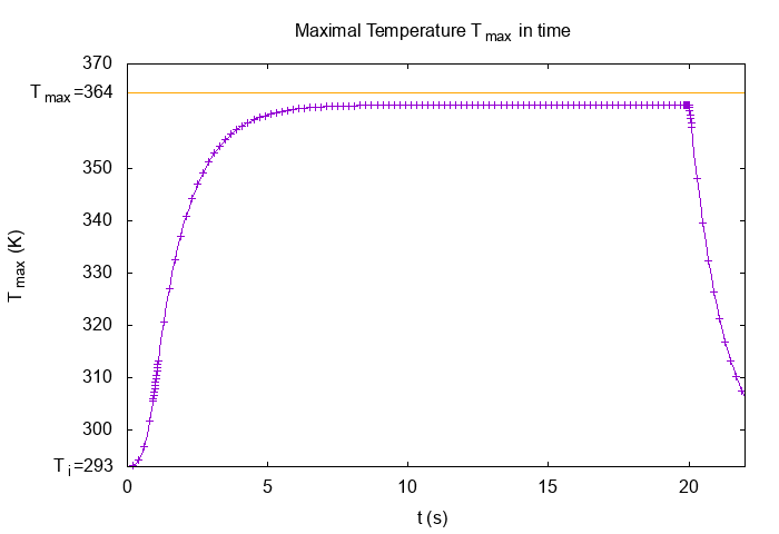
"a":1933.10, // K
"b":0.40041, // K
"rmax":0.0861910719118454, // m
"Tmax":364.446 // K
}
9. Coefficient Form PDEs
We use the application Coefficient Form PDEs. The coefficient associate to Weak Formulation are :
-
For Magnetic equation of unknow \(\mathbf{A}\) :
-
On
Conductor:
Coefficient
Description
Expression
\(d\)
damping or mass coefficient
\(\sigma\)
\(c\)
diffusion coefficient
\(\frac{1}{\mu}\)
\(f\)
source term
\(- \sigma \, \nabla V\)
-
On
Air:
Coefficient
Description
Expression
\(c\)
diffusion coefficient
\(\frac{r}{\mu}\)
-
-
For Electric equation of unknow \(\mathbf{A}\) :
-
On
Conductor:
Coefficient
Description
Expression
\(c\)
diffusion coefficient
\(\sigma\)
\(\gamma\)
source term
\(\sigma \mathbf{A}\)
-
-
For heat equation (Weak Heat Axis), on
Conductor(the temperature isn’t computed onAir) :Coefficient
Description
Expression
\(d\)
damping or mass coefficient
\(\rho \, C_p\)
\(c\)
diffusion coefficient
\(k\)
\(f\)
source term
\(\sigma \, \left( \nabla V + \frac{\partial \mathbf{A}}{\partial t} \right)\)
On JSON file, the coefficients are writed :
    "Materials":
    {
        "Conductor":
        {
            "sigma":58e6,       // S.m-1
            "mu":"4*pi*1e-7",   // kg.m/A2/S2

            "magnetic_d":"sigma:sigma",
            "magnetic_c":"1/mu:mu",
            "magnetic_f":"{-sigma*electric_grad_V_0,-sigma*electric_grad_V_1,-sigma*electric_grad_V_2}:sigma:electric_grad_V_0:electric_grad_V_1:electric_grad_V_2",

            "electric_c":"sigma:sigma",
            "electric_gamma":"{sigma*magnetic_dA_dt_0,sigma*magnetic_dA_dt_1,sigma*magnetic_dA_dt_2}:sigma:magnetic_dA_dt_0:magnetic_dA_dt_1:magnetic_dA_dt_2",

            "k":380,        // W/m/K
            "rho":10000,    // kg/m3
            "Cp":380,       // J/K/kg

            "heat_c":"k:k",
            "heat_f":"materials_Conductor_sigma*((electric_grad_V_0+magnetic_dA_dt_0)*(electric_grad_V_0+magnetic_dA_dt_0)+(electric_grad_V_1+magnetic_dA_dt_1)*(electric_grad_V_1+magnetic_dA_dt_1)+(electric_grad_V_2+magnetic_dA_dt_2)*(electric_grad_V_2+magnetic_dA_dt_2)):materials_Conductor_sigma:electric_grad_V_0:electric_grad_V_1:electric_grad_V_2:magnetic_dA_dt_0:magnetic_dA_dt_1:magnetic_dA_dt_2",
            "heat_d":"rho*Cp:rho:Cp"
        },
        "Air":
        {
            "physics":"magnetic",
            "mu":"4*pi*1e-7",   // kg.m/A2/S2
            "magnetic_c":"1/mu:mu"
        }
    }
10. Numeric Parameters
This section show the parameters used to compute the simulation.
-
Size of mesh : \(5 \, mm\)
-
Time Parameters :
-
Time step : I use adaptative time step. Near of brutal changement of current, the time step is little, in other case, the time step is big. I put adaptative time step to have good precision near of changement (cut of current at \(t=22s\)) and to not explose the time of compute. The shell script feelpp_adaptative.sh implements that.
\(\Delta_t = \left\{ \begin{matrix} 0.1s \, \text{for} \, 0s<t<0.9s \\ 0.008s \, \text{for} \, 0.9s<t<1.1s \\ 0.1s \, \text{for} \, 1.1s<t<19.9s \\ 0.008s \, \text{for} \, 19.9s<t<20.1s \\ 0.1 \, \text{for} \, 20.1s<t<22s \end{matrix} \right.\)
-
Initial Time : \(0 \, s\)
-
Final Time : \(22 \, s\)
-
-
Element type : \(P1\) for three equation (\(\mathbf{A}\), \(V\) and \(T\))
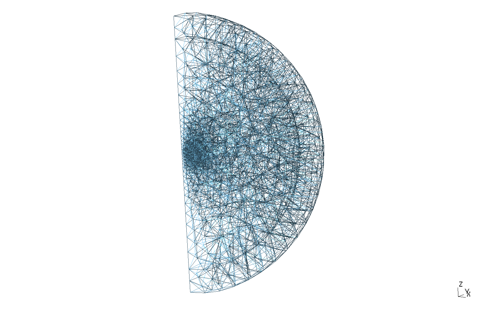
Mesh of Geometry
|
11. Exact solutions
11.1. Intensity
In this subsection, we see the analytical compute of intensity.
We have :
| In stationary case we have \(U = R \, I\). |
And :
-
Resolution of first part (\(0s \leq t \leq 1s\)) :
The homogenous equation \(R \, I_0 + L \, \frac{dI_0}{dt} = 0\) have a solve : \(I_0(t) = e^{-\frac{R}{L}t}\)
We pose \(C(t)\), such that \(I(t) = C(t) \, I_0(t) = C(t) \, e^{-\frac{R}{L}t}\) is solution of equation (Intensity-1).
Thus :
Thus :
-
Resolution of second part (\(1s \leq t \leq 20s\)) :
An evident solution is :
-
Resolution of third part (\(20s \leq t\)) :
An evident solution is :
To conclude, we have :
12. Result
The analytical solve of potential magnetic field and magnetic field (the cyan curve on plots) is computed by python3’s module MagnetTools.MagnetTools. The module based on paper : spire.
The analytical solve of intensity (and magnetic field) is computed on python3’s script Edit the file.
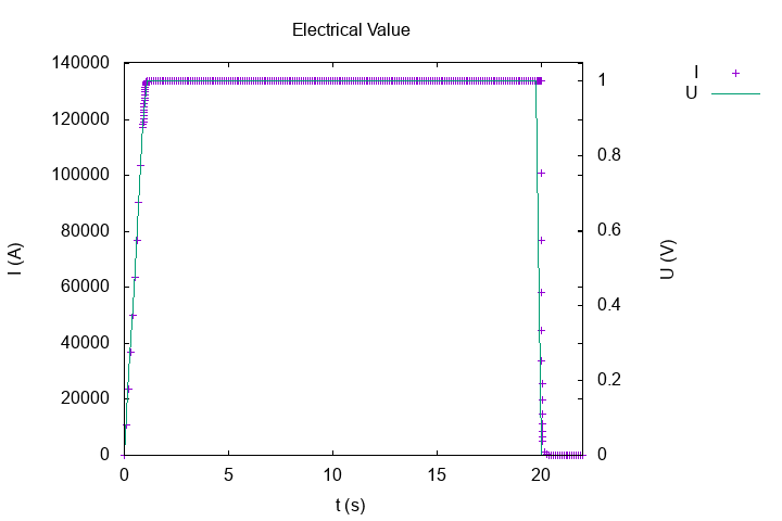
12.1. Intensity
Feelpp compute in post-process, the intensity of circuit :
The intensity verify the equation :
With \(R\) the resistance of torus of conductor and \(L\) the inductance of conductor.
In case of a rectangular cross section \((r_{int},r_{ext}) \times (z_1,z_2)\) torus, we can show that :
We have the value :
Symbol |
Description |
Value |
Unit |
R |
resistance of torus |
\(7.5313 \times 10^{-6}\) |
Ohm |
L |
inductance of torus |
\(1.9204 \times 10^{-7}\) |
Henry |
The exact solution is (see the subsection Intensity for more detail) :
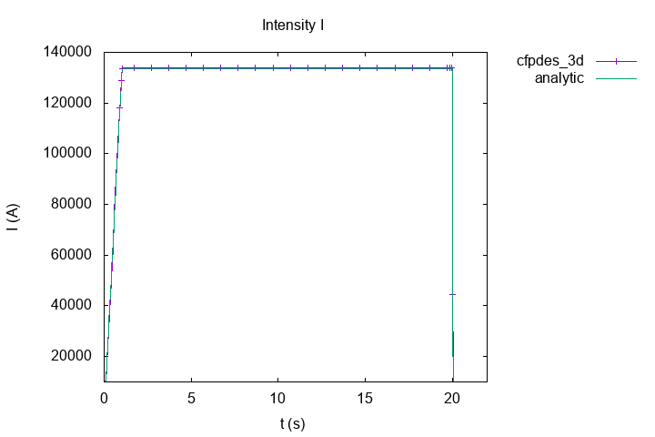
Intensity of current \(I(A)\)
|
In stationary case, we have the Ohm law :
With this relation, we have theorycal intensity : \(I_{th} = \frac{U}{R} = -132779 \, A\). And with numeric solve, we have \(I_{num} = -1.3376228966881469e+05 \, A\), so an error of \(7.4e-3 \, A\).
12.2. Magnetic field \(B_z\)
Recall, with axisymmetric condition :
Thus \(B_z = \frac{1}{r} \frac{\partial \Phi}{\partial r} \).
-
On \(Or\) axis at \(t=20s\)
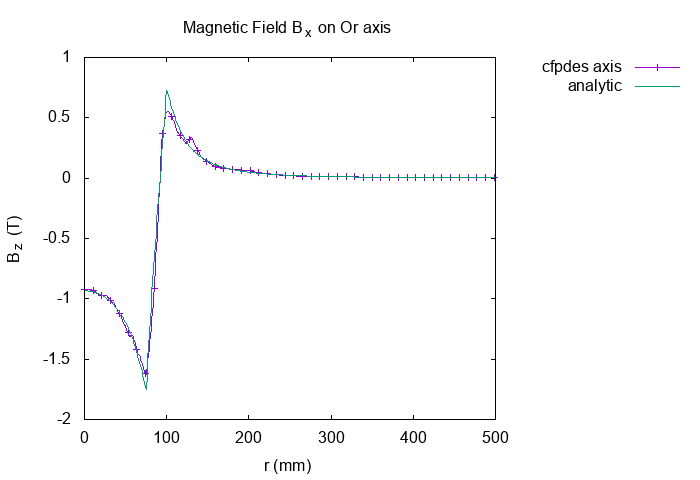
Horizontal Magnetic Field \(B_z(T)\) on Or
|
-
On origin \((0,0,0)\) across the time
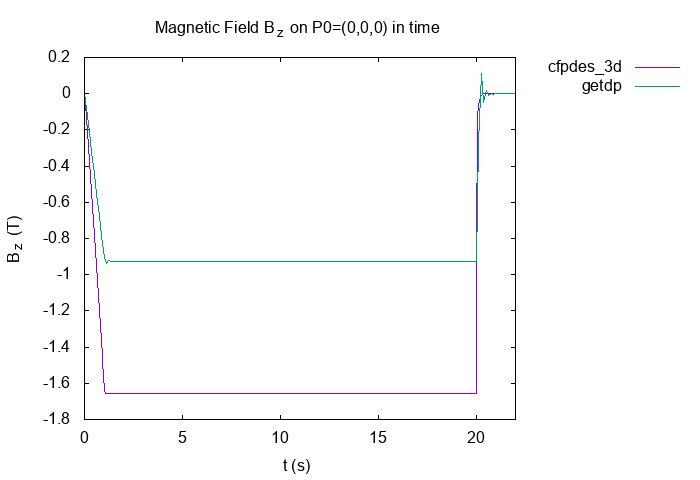
"Horizontal Magnetic Field \(B_z(T)\)
|
-
Magnetic Field across the time :
Horizontal Magnetic Field \(B_z(T)\)
|