Test Case of Elasto-Magnetism in Stationary and Axisymmetrical Case

1. Introduction

This page presents the simulation and result of page Elastic Equations with Electromagnetism and Thermic in Axisymmetrical case : Elastic and Electromagnetism problem coupled by Laplace Force in stationnary and axisymmetrical case.

2. Run the calculation

The command line to run this case is :

    mpirun -np 16 feelpp_toolbox_coefficientformpdes --config-file=elasto-thermo-mag.cfg --cfpdes.gmsh.hsize=5e-3

To compute with only the Laplace Force, please, put :

        "bool_laplace":1,
        "bool_dilatation":0,

On Parameter function of .json file elasto-thermo-mag.json.

3. Data Files

The case data files are available in Github here :

CFG file - Edit the file
JSON file - Edit the file
GEO file - Edit the file

4. Equation

In this subsection, we couple the equation (Static Elasticity Axis) of Elastic equation and (AV Axis) AV-Formulation in axisymmetrical coordinates.

The domain of resolution of electromagnetism part is \(\Omega^{axis}\) with bounds \(\Gamma^{axis}\), \(\Gamma_D^{axis}\) the bound of Dirichlet conditions and \(\Gamma_N^{axis}\) the bound of Neumann conditions such that \(\Gamma^{axis} = \Gamma_N^{axis} \cup \Gamma_D^{axis}\).

The domain of resolution of elastic part is \(\Omega_c^{axis} \subset \Omega^{axis}\) (and the domain of definition of electrical potential \(V\) and electrical conductivity \(\sigma\)) with bounds \(\Gamma_c^{axis}\), \(\Gamma_{D \hspace{0.05cm} elas}^{axis}\) the bound of Dirichlet conditions and \(\Gamma_{N \hspace{0.05cm} elas}^{axis}\) the bound of Neumann conditions such that \(\Gamma_c^{axis} = \Gamma_{D \hspace{0.05cm} elas}^{axis} \cup \Gamma_{N \hspace{0.05cm} elas}^{axis}\). The domain \(\Omega_c^{axis}\) correspond to the conductor.

Differential Formulation of Coupled Elasticity Equation and AV-Formulation in Stationary and Axisymmetrical case

\[\text{(Elasticity-AV Axis Static)} \\ \left\{ \begin{matrix} - \frac{1}{\mu} \Delta \Phi + \frac{2}{\mu \, r} \frac{\partial \Phi}{\partial r} + \sigma \frac{\partial V}{\partial \theta} = 0 & \text{ on } \Omega^{axis} & \text{(AV-1 Axis)} \\ \frac{\partial^2 V}{\partial \theta^2} = 0 & \text{ on } \Omega_c^{axis} & \text{(AV-2 Axis)} \\ - \nabla \cdot \bar{\bar{\sigma}} = \mathbf{F}_{laplace} & \text{on } \Omega_c^{axis} & \text{(Elas-1)} \\ A_{\theta} = 0 & \text{ on } \Gamma_D^{axis} & \text{(D Axis)} \\ \frac{\partial A_{\theta}}{\partial \mathbf{n}^{axis}} = 0 & \text{ on } \Gamma_N^{axis} & \text{(N Axis)} \\ \mathbf{u} = 0 & \text{on } \Gamma_{D \hspace{0.05cm} elas}^{axis} & \text{(D elas)} \\ \bar{\bar{\sigma}} \cdot \mathbf{n} = 0 & \text{on } \Gamma_{N \hspace{0.05cm} elas}^{axis} & \text{(N elas)} \end{matrix} \right.\]

With :

Lamé’s coefficients : \(\lambda = \frac{E \, v}{(1-2 v) \, (1+v)}\), \(\mu = \frac{E}{2 \, (1+v)}\) with
- Young modulus \(E\)
- Poisson’s coefficient \(v\)

Magnetic potential field : \(\mathbf{A}\) thus :
- \(\mathbf{B}=\nabla \times \mathbf{A}\)
- \(\Phi = r \, A_{\theta}\)

Displacement \(\mathbf{u} = \begin{pmatrix} u_x \\ u_y \\ u_z \end{pmatrix}\)

Electric Potential Scalar : \(V\)

Stress Tensor with Hooke Law : \(\bar{\bar{\sigma}} = \bar{\bar{\sigma}}^E = \lambda \, Tr(\bar{\bar{\epsilon}})+2\mu \bar{\bar{\epsilon}}\)

Electrical conductivity : \(\sigma\)

Laplace Force : \(\mathbf{F}_{Laplace} = \begin{pmatrix} \frac{1}{r} j_{\theta} \frac{\partial \Phi}{\partial r} \\ 0 \\ \frac{1}{r} j_{\theta} \frac{\partial \Phi}{\partial z} \end{pmatrix}_{cyl}\)

And notations :

Divergence of tensor : \(\nabla \cdot \bar{\bar{\sigma}} = \begin{pmatrix} \nabla \cdot \bar{\bar{\sigma}}_{r,:} + \frac{\bar{\bar{\sigma}}_{rr} - \bar{\bar{\sigma}}_{\theta \theta}}{r} \\ \nabla \cdot \bar{\bar{\sigma}}_{z,:} + \frac{\bar{\bar{\sigma}}_{rz}}{r} \end{pmatrix}\)
Scalar produce of tensor : \(\bar{\bar{\sigma}} \cdot \mathbf{n} = \begin{pmatrix} \bar{\bar{\sigma}}_{r,:} \cdot \mathbf{n}^{axis} \\ \bar{\bar{\sigma}}_{z,:} \cdot \mathbf{n}^{axis} \end{pmatrix} = \begin{pmatrix} \bar{\bar{\sigma}}_{rr} \, n_r + \bar{\bar{\sigma}}_{rz} \, n_z \\ \bar{\bar{\sigma}}_{zr} \, n_r + \bar{\bar{\sigma}}_{zz} \, n_z\end{pmatrix}\)

The equation become coupled in one senses, the second equation (Elas-1 Axis) depends of potentials.

We don’t care of geometrical deformation which can change the mesh or the density. We suppose the geometry is fixed.

5. Geometry

The geometry is a torus of the conductor in cartesian coordinates \((x,y,z)\) or rectangle in axisymmetric coordinates \((r,z)\), surrounded by air.

Geometry in axisymmetrical cut loop on Conductor

Geometry in axisymmetrical cut

Geometry in three dimensions

Geometry in three dimensions cut loop on Conductor

The geometrical domains are :

Conductor : the torus is composed by conductor material
- Interior : interior surface of conductor ring
- Exterior : exterior surface of conductor ring
- Upper : upper of conductor ring
- Bottom : bottom of conductor ring
Air : the air surround Conductor
- zAxis : a bound of Air, correspond to \(Oz\) axis (\(\{(z,r), \, z=0 \}\))
- infty : the rest of bound of Air

Symbol

Description

value

unit

\(r_{int}\)

interior radius of torus

\(75e-3\)

\(r_{ext}\)

exterior radius of torus

\(100.2e-3\)

\(z_1\)

half-height of torus

\(300e-3\)

\(r_{infty}\)

radius of infty border

\(5*r_{ext}\)

6. Boundary Conditions

We impose the boundary conditions :

Magnetic Equation :
- Strong Dirichlet :
  - On zAxis : \(\Phi = 0\) (\(A_{\theta} = 0\) by symetric argument)
  - On infty : \(\Phi = 0\) (\(A_{\theta} = 0\) we consider the bound of resolution like infty for magnetic field)
Heat Equation :
- Neumann : \(\frac{\partial T}{\partial \mathbf{n}} = 0\) on Interior and Exterior
- Robin : \(-k \, \frac{\partial T}{\partial \mathbf{n}} = h \, \left( T - T_c \right)\) on Upper and Bottom. The Robin condition represents the cooling by water.
Elastic Equation :
- Strong Dirichlet : \(\mathbf{u} = 0\) on Upper and Bottom. The Dirichlet condition represents the embedding of mechanical part.
- Neumann : \(\bar{\bar{\sigma}} \cdot \mathbf{n} = 0\) on Interior and Exterior. The Neumann condition represents the freedom of displacement.

On JSON file, the boundary conditions are writed :

Boundary conditions on JSON file

    "BoundaryConditions":
    {
        "magnetic":
        {
            "Dirichlet":
            {
                "magdir":
                {
                    "markers":["ZAxis","Infty"],
                    "expr":"0"
                }
            }
        },
        "heat":
        {
            "Robin":
            {
                "heatdir":
                {
                    "markers":["Interior","Exterior"],
                    "expr1":"h*x:h:x",
                    "expr2":"h*T_c*x:h:T_c:x"
                }
            }
        },
        "elastic":
        {
            "Dirichlet":
            {
                "elasdir":
                {
                    "markers":["Upper","Bottom"],
                    "expr":"{0,0}"
                }
            }
        }
    }

7. Weak Formulation

We obtain :

Weak Formulation of Elastic Thermic Electromagnetism equations in Axisymmetric and Stationnary Case Vectorial

\[\tiny{ \text{(Weak Thermo-Mag Axis Static)} \\ \left\{ \begin{eqnarray*} \int_{\Omega^{axis}}{ \frac{1}{\mu} \tilde{\nabla} \Phi \cdot \tilde{\nabla} \mathbf{ϕ} \ r \ drdz } + \int_{\Omega^{axis}}{\frac{2}{\mu \, r} \frac{\partial \Phi}{\partial r} \, \mathbf{ϕ} \ r \ drdz} = - \int_{\Omega_c^{axis}}{ \sigma \frac{\partial V}{\partial \theta} \mathbf{ϕ} \ r \ drdz } & \text{(Weak AV Axis)} \\ \int_{\Omega_c^{axis}}{ k \, \tilde{\nabla} T \cdot \tilde{\nabla} \mathbf{ϕ} \, r \, drdz } + \int_{\Gamma_R^{axis}}{ h \, T \, \mathbf{ϕ} \, r \, d\Gamma } = \int_{\Omega_c^{axis}}{ Q \, \mathbf{ϕ} \, r \, drdz } + \int_{\Gamma_R^{axis}}{ h \, T_c \, \mathbf{ϕ} \, r \, d\Gamma } & \text{(Weak Heat Axis)} \\ \int_{\Omega_c^{axis}} \left( r \left( \lambda \left( \frac{\partial u_r}{\partial r} + \frac{1}{r} u_r + \frac{\partial u_z}{\partial z} \right) \right) \left( \frac{\partial \xi_r}{\partial r} + \frac{1}{r} \xi_r \right) + r \mu \left[ 2 \left( \frac{\partial u_r}{\partial r} \frac{\partial \xi_r}{\partial r} + \frac{1}{r^2} u_r \xi_r \right) + \left( \frac{\partial u_r}{\partial z} \frac{\partial \xi_r}{\partial z} + \frac{\partial u_z}{\partial r} \frac{\partial \xi_r}{\partial z} \right) \right] \\ + r \mu \left( \frac{\partial u_r}{\partial z} + \frac{\partial u_z}{\partial r} \right) \frac{\partial \xi_z}{\partial r} + r \left[ \lambda \left( \frac{\partial u_r}{\partial r} + \frac{1}{r} u_r + \frac{\partial u_z}{\partial z} \right) + 2\mu \frac{\partial u_z}{\partial z} \right] \frac{\partial \xi_z}{\partial z} \right) dr dz \\ = \int_{\Omega_c^{axis}}{r \, \mathbf{F}_{laplace} \cdot \mathbf{ξ} \ dr dz} + \int_{\Gamma_{N \hspace{0.05cm} elas}^{axis}}{ r \, \mathbf{g} \cdot \mathbf{ξ} \ dr dz } + \int_{\Gamma_{R \hspace{0.05cm} elas}^{axis}}{ r \left( \mathbf{g} - k \mathbf{u} \right) \cdot \mathbf{ξ} \ dr dz } & \hspace{0.5cm} \text{(Weak Static Elasticity Axis)} \\ \text{for } \mathbf{ϕ} \in H^1(\Omega)^2, \ \psi \in H^1(\Omega_c) , \ \eta \in H^1(\Omega_c), \ \mathbf{ξ} = \begin{pmatrix} xi_x \\ \xi_y \\ \xi_z \end{pmatrix} \in H^1(\Omega_c)^2 \ \text{and} \ \mathbf{F}_{laplace} = \begin{pmatrix} F_{laplace \, r} \\ 0 \\ F_{laplace \, z} \end{pmatrix} = \begin{pmatrix} - \frac{\sigma}{r^2} \frac{\partial V_{\theta}}{\partial \theta} \frac{\partial \Phi}{\partial r} \\ 0 \\ - \frac{\sigma}{r^2} \frac{\partial V_{\theta}}{\partial \theta} \frac{\partial \Phi}{\partial z} \end{pmatrix}_{cyl} \end{eqnarray*} \right. }\]

8. Parameters

The parameters of problem are :

On Conductor :

Symbol

Description

Value

Unit

\(V\)

scalar electrical potential

\( U \, \frac{\theta}{2\pi}\)

\(Volt\)

\(U\)

electrical potential

\(0.2\)

\(Volt\)

\(\sigma\)

electrical conductivity at \(T=T_0\)

\(58e6\)

\(S/m\)

\(j_{\theta}\)

orthoradial current density

\(- \sigma \frac{U}{2\pi} \, \frac{1}{r}\)

\(A/m^2\)

\(E\)

Young Modulus

\(2.1e6\)

\(Pa\)

\(v\)

Poisson’s coefficient

\(0.33\)

\(dimensionless\)

\(\lambda\)

Lame’s coefficient

\(\frac{E \, v}{(1-2v)(1+v)}\)

\(Pa\)

\(\mu\)

Lame’s coefficient

\(\frac{E}{2 (1+v)}\)

\(Pa\)

On Air :

Symbol

Description

Value

Unit

\(\mu=\mu_0\)

magnetic permeability of vacuum

\(4\pi.10^{-7}\)

\(kg \, m / A^2 / S^2\)

On JSON file, the parmeters are writed :

Parameters on JSON file

    "Parameters":
    {
        "bool_laplace":1,
        "bool_dilatation":0,

        "h":80000,      // W/m2/K
        "T_c":293,      // K
        "T0":293,       // K

        // Constants of analytical solve
        "a":77.32,      // K
        "b":0.40041,    // K
        "rmax":0.0861910719118454,  // m
        "Tmax":295.85   // K
    }

9. Coefficient Form PDEs

We use the application Coefficient Form PDEs. The coefficient associate to Weak Formulation are :

For MQS equation (Weak MQS Axis) :

On Conductor :

Coefficient

Description

Expression

\(d\)

damping or mass coefficient

\(\sigma\)

\(c\)

diffusion coefficient

\(\frac{r}{\mu}\)

\(\beta\)

convection coefficient

\(\begin{pmatrix} \frac{2}{\mu} \\ 0 \end{pmatrix}\)

\(f\)

source term

\(j_{\theta} \, r^2\)

On Air :

Coefficient

Description

Expression

\(c\)

diffusion coefficient

\(\frac{r}{\mu}\)

For heat equation, on Conductor (the temperature isn’t computed on Air)

Coefficient

Description

Expression

\(d\)

damping or mass coefficient

\(\rho \, C_p\)

\(c\)

diffusion coefficient

\(k\)

\(f\)

source term

\(- \sigma \left( \frac{U}{2\pi \, r} \right)^2\)

For elastic equation, on Conductor (the displacement isn’t computed on Air) :

Coefficient

Description

Expression

\(c\)

diffusion coefficient

\(r \mu\)

\(\gamma\)

conservative flux source term

\(\begin{pmatrix} - \lambda \left( r \frac{\partial u_r}{\partial r} + u_r + r \frac{\partial u_z}{\partial z} \right) - \mu \, r \, \frac{\partial u_r}{\partial r} & - \mu \, r \, \frac{\partial u_z}{\partial r} \\ - \mu \, r \, \frac{\partial u_r}{\partial z} & - \lambda \left( r \, \frac{\partial u_r}{\partial r} + u_r + r \, \frac{\partial u_z}{\partial z} \right) - \mu \, r \, \frac{\partial u_z}{\partial z} \end{pmatrix}\)

\(f\)

source term

\(\begin{pmatrix} r F_r - \lambda \frac{\partial u_r}{\partial r} - (\lambda+2\mu) \frac{u_r}{r} - \lambda \frac{\partial u_z}{\partial z} \\ r F_z \end{pmatrix}\)

On JSON file, the coefficients are writed :

CFPDEs coefficients on JSON file

   "Materials":
    {
        "Conductor":
        {
            // Magnetic Part
            "U":0.2,            // Volt
            "sigma":58e+6,      // S.m-1
            "mu":"4*pi*1e-7",   // kg.m/A2/S2

            "j_th":"-sigma*U/2/pi/x:sigma:U:x",

            "magnetic_c":"x/mu:x:mu",
            "magnetic_beta":"{2/mu,0}:mu",
            "magnetic_f":"-sigma*U/2/pi*x:sigma:U:x",

            // Heat Part
            "k":380,            // W/m/K
            "heat_c":"k*x:k:x",
            "heat_f":"sigma*U/(2*pi)*U/(2*pi)/x:sigma:U:x",

            // Elastic Part
            "E":2.1e6,          // Pa
            "v":0.33,           // dimensionless
            "alpha_T":"17e-6",  // K-1

            "Lame_lambda":"E*v/(1-2*v)/(1+v):E:v",
            "Lame_mu":"E/(2*(1+v)):E:v",

            "F_laplace":"{1/x*j_th*magnetic_grad_phi_0, 1/x*j_th*magnetic_grad_phi_1}::x:j_th:magnetic_grad_phi_0:magnetic_grad_phi_0:magnetic_grad_phi_1",
            "sigma_T":"-(3*Lame_lambda+2*Lame_mu)*alpha_T*(heat_T-T0):Lame_lambda:Lame_mu:alpha_T:heat_T:T0",

            "elastic_c":"x*Lame_mu:x:Lame_mu",
            "elastic_gamma":"{-Lame_lambda*(x*elastic_grad_u_00+elastic_u_0+x*elastic_grad_u_11)-x*Lame_mu*elastic_grad_u_00-bool_dilatation*x*sigma_T, -x*Lame_mu*elastic_grad_u_10, -x*Lame_mu*elastic_grad_u_01, -Lame_lambda*(x*elastic_grad_u_00+elastic_u_0+x*elastic_grad_u_11)-x*Lame_mu*elastic_grad_u_11-bool_dilatation*x*sigma_T}:bool_dilatation:x:Lame_lambda:Lame_mu:elastic_u_0:elastic_grad_u_00:elastic_grad_u_01:elastic_grad_u_10:elastic_grad_u_11:sigma_T",
            "elastic_f":"{bool_laplace*x*F_laplace_0-Lame_lambda*elastic_grad_u_00-(Lame_lambda+2*Lame_mu)*elastic_u_0/x-Lame_lambda*elastic_grad_u_11-bool_dilatation*sigma_T, bool_laplace*x*F_laplace_1}:bool_laplace:bool_dilatation:x:F_laplace_0:F_laplace_1:Lame_mu:Lame_lambda:elastic_u_0:elastic_grad_u_00:elastic_grad_u_01:elastic_grad_u_11:sigma_T",

            "sigma_rr":"(Lame_lambda+2*Lame_mu)*elastic_grad_u_00+Lame_lambda*elastic_u_0/x+Lame_lambda*elastic_grad_u_11+bool_dilatation*sigma_T:bool_dilatation:Lame_lambda:Lame_mu:x:elastic_u_0:elastic_grad_u_00:elastic_grad_u_11:elastic_grad_u_22:sigma_T",
            "sigma_thth":"Lame_lambda*elastic_grad_u_00+(Lame_lambda+2*Lame_mu)*Lame_lambda*elastic_u_0/x+Lame_lambda*elastic_grad_u_11+bool_dilatation*sigma_T:bool_dilatation:Lame_lambda:Lame_mu:x:elastic_u_0:elastic_grad_u_00:elastic_grad_u_11:elastic_grad_u_22:sigma_T",
            "sigma_zz":"Lame_lambda*elastic_grad_u_00+Lame_lambda*Lame_lambda*elastic_u_0/x+(Lame_lambda+2*Lame_mu)*elastic_grad_u_11+bool_dilatation*sigma_T:bool_dilatation:Lame_lambda:Lame_mu:x:elastic_u_0:elastic_grad_u_00:elastic_grad_u_11:elastic_grad_u_22:sigma_T",
            "sigma_rz":"Lame_mu*(elastic_grad_u_01+elastic_grad_u_10):Lame_mu:elastic_grad_u_01:elastic_grad_u_10",

            "sigma_1":"Lame_lambda/x*elastic_u_0+(Lame_lambda+Lame_mu)*(elastic_grad_u_00+elastic_grad_u_11)+bool_dilatation*sigma_T+Lame_mu*sqrt((elastic_grad_u_00-elastic_grad_u_11)*(elastic_grad_u_00-elastic_grad_u_11)+4*(elastic_grad_u_01+elastic_grad_u_10)*(elastic_grad_u_01+elastic_grad_u_10)):bool_dilatation:x:Lame_lambda:Lame_mu:elastic_u_0:elastic_grad_u_00:elastic_grad_u_11:elastic_grad_u_01:elastic_grad_u_10:sigma_T",
            "sigma_2":"Lame_lambda*elastic_grad_u_00+(Lame_lambda+2*Lame_mu)/x*elastic_u_0+Lame_lambda*elastic_grad_u_11+bool_dilatation*sigma_T:bool_dilatation:x:Lame_lambda:Lame_mu:elastic_u_0:elastic_grad_u_00:elastic_grad_u_11:sigma_T",
            "sigma_3":"Lame_lambda/x*elastic_u_0+(Lame_lambda+Lame_mu)*(elastic_grad_u_00+elastic_grad_u_11)+bool_dilatation*sigma_T-Lame_mu*sqrt((elastic_grad_u_00-elastic_grad_u_11)*(elastic_grad_u_00-elastic_grad_u_11)+4*(elastic_grad_u_01+elastic_grad_u_10)*(elastic_grad_u_01+elastic_grad_u_10)):bool_dilatation:x:Lame_lambda:Lame_mu:elastic_u_0:elastic_grad_u_00:elastic_grad_u_11:elastic_grad_u_01:elastic_grad_u_10:sigma_T"
        },
        "Air":
        {
            "physics":"magnetic",
            "mu":"4*pi*1e-7",   // kg.m/A2/s2
            "magnetic_c":"x/mu:x:mu",
            "magnetic_beta":"{2/mu,0}:mu"
        }
    }

10. Numeric Parameters

Mesh size :
- Interior of torus : \(0.01 m\)
- Far from the torus : \(0.2 m\)
Element Type : I run the simulation in \(P_2\) elements.

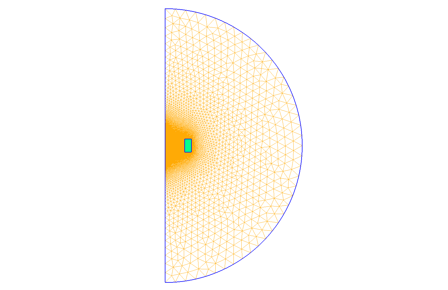
Mesh of Geometry

11. Exact solutions

11.1. Displacement on Or axis

The calculus is based on book Solenoid Magnet Design but it presents an error.

11.1.1. Approximations

We want to compute exactly the displacement on \(r=0\), for that, we suppose that the height is infinitely great. The elastic equations is reduced in its r-component :

\[ - \bar{\bar{\sigma}}_{\theta \theta} + \frac{\partial \left( r \bar{\bar{\sigma}}_{rr} \right)}{\partial r} = - r \, J_{\theta} \, B_z\]

The z component of displacement is null : \(u_z = 0\).

And the stress tensor :

\[\begin{eqnarray*} \bar{\bar{\sigma}}_{rr} &=& \frac{E}{(1-2 v)(1+v)} \left( (1-v) \frac{\partial u_r}{\partial r} + v \frac{u_r}{r} \right) \\ \bar{\bar{\sigma}}_{\theta \theta} &=& \frac{E}{(1-2 v)(1+v)} \left( v \frac{\partial u_r}{\partial r} + (1-v) \frac{u_r}{r} \right) \end{eqnarray*}\]

And \(\sigma_{zz} = \sigma_{rz} = 0\).

Thus, the elastic equation is writed :

\[ \frac{\partial}{\partial r} \left( r \frac{\partial u_r}{\partial r} \right) - \frac{u_r}{r} = - \frac{(1+v)(1-2v)}{E (1-v)} \, r \, J_{\theta} \, B_z\]

The solve \(u_r\) can be write in this form :

\[ u_r(r) = C_1 \, r + \frac{C_2}{r} + u_{pr}(r)\]

With \(C_1\), \(C_2\) two constants and \(u_{pr}\) a particular solve.

11.1.2. Compute of \(B_z\)

To compute \(u_{pr}\), we must to compute the magnetic field \(B\).

With the supposition of infinitely height, the r-component \(B_r\) is null \(B_r = 0\) and z-component depend uniquely of r \(B_z=B_z(r)\).

The Ampère Theorem gives us :

\[ \int_{C}{\mathbf{B} \cdot d \mathbf{l}} = \frac{1}{\mu} \, \int_{S}{ \mathbf{J} \cdot \mathbf{n} d S}\]

With \(S\) an any surface and \(C\) its bound.

We take \(S\) a square center in Or axis.

We have :

\[ B_z(r_{int}) - B_z(r) = \frac{1}{\mu} \, \int_{\tau=r_{int}}^{r}{ J_{\theta}(\tau) \, d\tau }\]

The distribution of current density \(J_{\theta}\) of magnet is of the form : \(J_{\theta} = J_{int} \, \frac{r_{int}}{r}\) with \(J_{int} = J_{\theta}(r_{int})\).

For this problem, we have \(J_{\theta} = \frac{U}{2\pi} \, \frac{1}{r}\).

It give :

\[ B_z(r) = B_z(r_{int}) - \frac{\Delta B_z}{ln(r_{ext}/r_{int})} \, ln(\frac{r}{r_{int}})\]

With \(\Delta B_z = B_z(r_{int}) - B_z(r_{ext})\)

11.1.3. Compute of \(u_{pr}\)

\(u_{pr}\) verify :

\[ \frac{\partial }{\partial r} \left( r \frac{\partial u_{pr}}{\partial r} \right) - \frac{u_{pr}}{r} = - \frac{(1+v)(1-2v)}{E (1-v)} \, r \, J_{\theta} \, B_z\]

With current density magnet distribution \(J_{\theta} = J_{int} \, \frac{r_{int}}{r}\) :

\[ \frac{\partial}{\partial r} \left( r \frac{\partial u_{pr}}{\partial r} \right) - \frac{u}{r} = - \frac{(1+v)(1-2v)}{E (1-v)} J_{int} r_{int} \left( \frac{\Delta B_z}{ln(r_{ext}/r_{int})} \, ln(\frac{r}{r_{int}}) \right)\]

It give :

\[ u_{pr}(r) = \frac{(1+v)(1-2v)}{E (1-v)} \, J_{int} r_{int} \, \frac{1}{4} \, r ln(\frac{r}{r_{int}}) \left[ \frac{\Delta Bz}{ln(r_{ext}/r_{int})} \, ln(\frac{r}{r_{int}}) - 2 B_z(r_{int}) + \frac{\Delta B_z}{ln(r_{ext}/r_{int})} \right]\]

Or :

\[ u_{pr}(r) = - \frac{(1+v)(1-2v)}{E (1-v)} \, J_{int} r_{int} \, \frac{1}{4} \, r ln(\frac{r}{r_{int}}) \left[ B_z(r) + B_z(r_{int}) + \frac{\Delta B_z}{ln(r_{ext}/r_{int})} \right]\]

11.1.4. Compute of constants

Nox, we introduce the boundary conditions. We have Neumann condition on \(r=r_{int}\) and \(r=r_{ext}\) :

\[\begin{eqnarray*} \sigma_{rr}(r_{int}) = 0 \\ \sigma_{rr}(r_{ext}) = 0 \end{eqnarray*}\]

With the expression of \(u\) :

\[\begin{eqnarray*} C_1 + (2v-1) \frac{C_2}{r_{int}^2} + (1-v) \frac{\partial u_r(r_{int})}{\partial r} + v \frac{u_r(r_{int})}{r_{int}} &=& 0 \\ C_1 + (2v-1) \frac{C_2}{r_{ext}^2} + (1-v) \frac{\partial u_r(r_{ext})}{\partial r} + v \frac{u_r(r_{ext})}{r_{ext}} &=& 0 \end{eqnarray*}\]

We obtain :

\[\begin{eqnarray*} C_1 &=& \frac{1}{r_{int}^2-r_{ext}^2} \left( r_{ext}^2 \left( (1-v) \frac{\partial u_r}{\partial r}(r_{ext}) + v \frac{u_r(r_{ext})}{r_{ext}} \right) - r_{int}^2 \left( (1-v) \frac{\partial u_r}{\partial r}(r_{int}) + v \frac{u_r(r_{int})}{r_{int}} \right) \right) \\ C_2 &=& \frac{1}{2v-1} \frac{r_{int}^2 r_{ext}^2}{r_{int}^2-r_{ext}^2} \left( (1-v) \frac{\partial u_r}{\partial r}(r_{int}) + v \frac{u_r(r_{int})}{r_{int}} - (1-v) \frac{\partial u_r}{\partial r}(r_{ext}) - v \frac{u_r(r_{ext})}{r_{ext}} \right) \end{eqnarray*}\]

11.1.5. Conclusion

The exact solution of elastic equation for infinitely height is :

\[\left\{ \begin{eqnarray*} u_r(r) &=& C_1 \, r + \frac{C_2}{r} + u_{pr}(r) \\ u_{pr}(r) &=& - \frac{(1+v)(1-2v)}{E (1-v)}\, J_{int} r_{int} \, \frac{1}{4} \, r ln(\frac{r}{r_{int}}) \left[ B_z(r) + B_z(r_{int}) + \frac{\Delta B_z}{ln(r_{ext}/r_{int})} \right] \\ C_1 &=& \frac{1}{r_{int}^2-r_{ext}^2} \left( r_{ext}^2 \left( (1-v) \frac{\partial u_r}{\partial r}(r_{ext}) + v \frac{u_r(r_{ext})}{r_{ext}} \right) - r_{int}^2 \left( (1-v) \frac{\partial u_r}{\partial r}(r_{int}) + v \frac{u_r(r_{int})}{r_{int}} \right) \right) \\ C_2 &=& \frac{1}{2v-1} \frac{r_{int}^2 r_{ext}^2}{r_{int}^2-r_{ext}^2} \left( (1-v) \frac{\partial u_r}{\partial r}(r_{int}) + v \frac{u_r(r_{int})}{r_{int}} - (1-v) \frac{\partial u_r}{\partial r}(r_{ext}) - v \frac{u_r(r_{ext})}{r_{ext}} \right) \end{eqnarray*} \right.\]

12. Result

12.1. Displacements

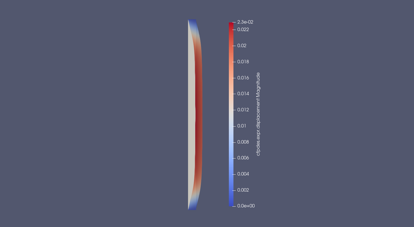
Deformation due to Thermal Dilatation Force : The white solid is initial geometry and the coloured solid is the final geometry (the colours represent Magnitude of displacement \(u (m)\))

The Thermal Dilatation deform the cylinder like a barrel filled with water. The cylinder deforms outwards.

We can note that near of embeded (Upper and Bottom), the cylinder deforms inwards.

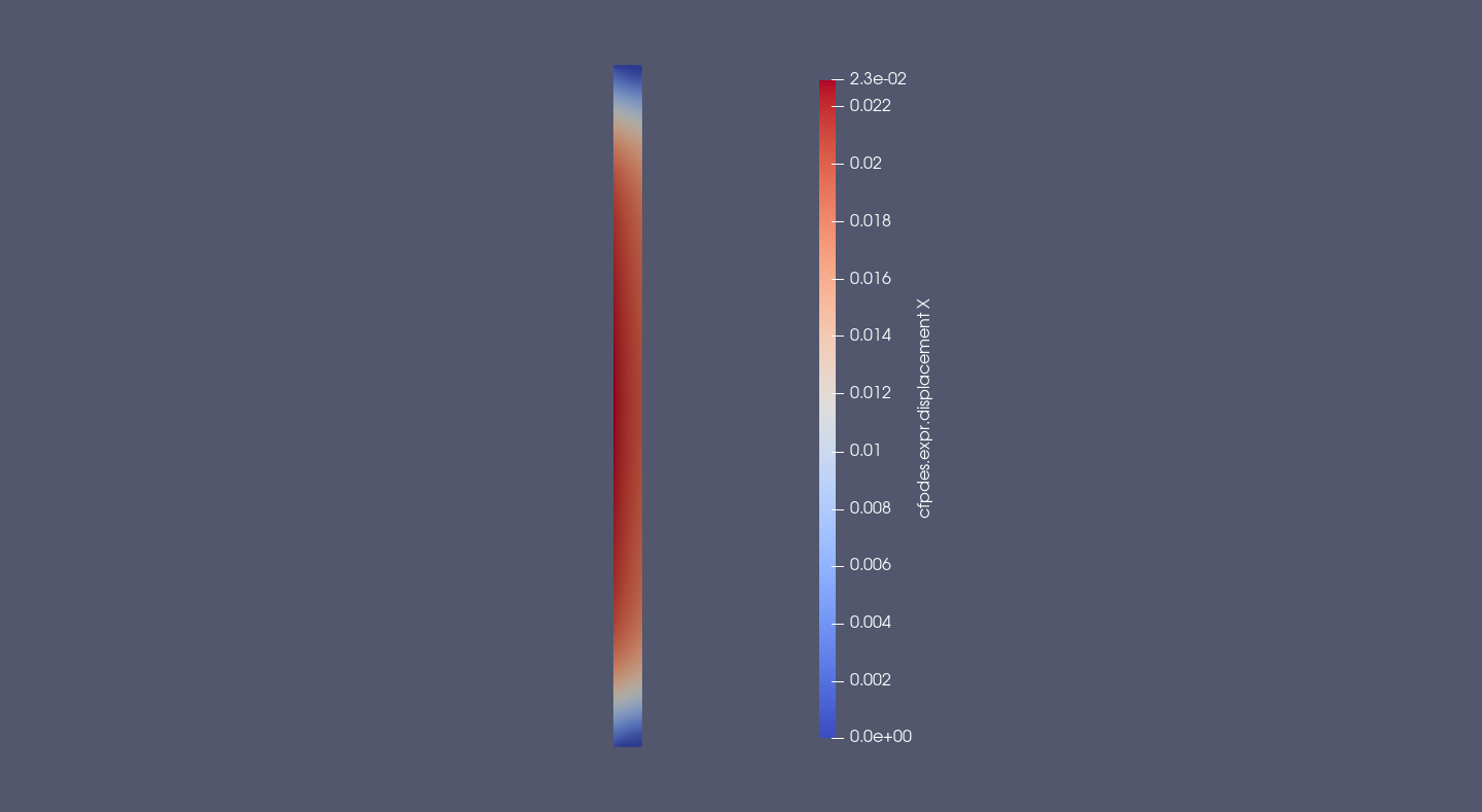
\(u_r(m)\)

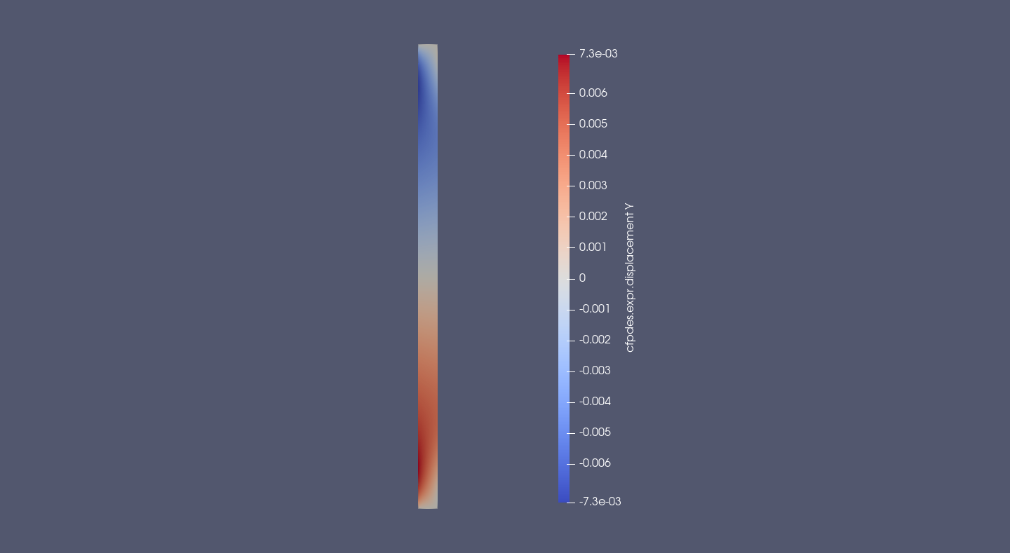
\(u_z(m)\)

The radial displacement \(u_r\) is maximum on Or axis near of the interior and decreases to zeros near of the embedded (on Upper and Bottom).

The z-displacement is symmetric by Or axis. Near of the interior, it positive in bottom part and negativ to upper part, the cylinder compresses toward the Or axis in z-displacement.

12.2. Tensor of Deformation \(\bar{\bar{\epsilon}}\)

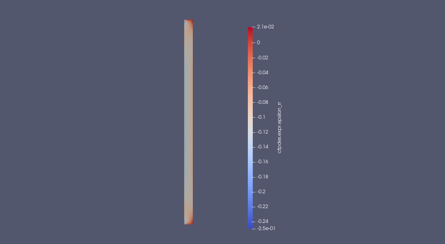
\(\bar{\bar{\epsilon}}_{rr} = \frac{\partial u_r}{\partial z}\)

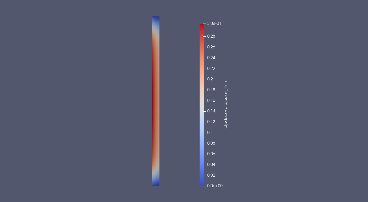
\(\bar{\bar{\epsilon}}_{\theta \theta} = \frac{1}{r} \, u_r\)

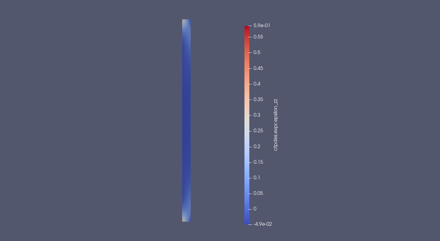
\(\bar{\bar{\epsilon}}_{zz} = \frac{\partial u_z}{\partial z}\)

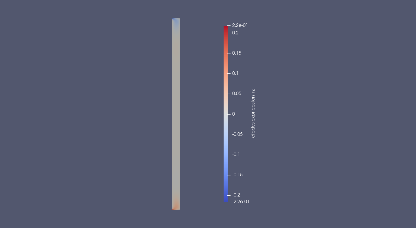
\(\bar{\bar{\epsilon}}_{rz} = \frac{1}{2} \left( \frac{\partial u_r}{\partial z} + \frac{\partial u_z}{\partial r} \right)\)

The radial deformation is uniform by z. It maximum on middle radius (\(\frac{r_{int}+r_{ext}}{2} \approx 87 mm\))

The orthoradial deformation is the greatest contribution of deformation. It maximum in Or axis near of the interior and decrease to negative value near of embedding (Upper and Bottom).

The z-deformation near of the center is symetric by Oz axis. The cylinder compresses near of the interior and it expands near of the exterior.

The rz-shear is great around the embededding and null in the rest of cylinder.

12.3. Stress Tensor \(\bar{\bar{\sigma}}\)

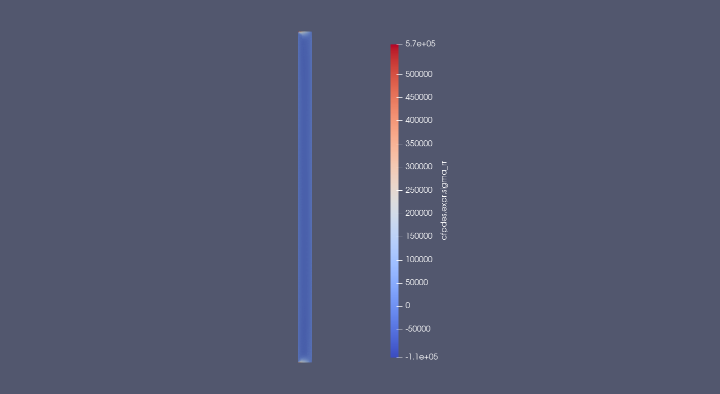
\(\scriptsize{\bar{\bar{\sigma}}_{rr} = \frac{\lambda}{r} \, u_r + \left( \lambda + 2\mu \right) \, \frac{\partial u_r}{\partial r} + \lambda \, \frac{\partial u_z}{\partial z} - (3\lambda + 2\mu) \, \alpha_T \, \left(T-T_0\right) (Pa)}\)

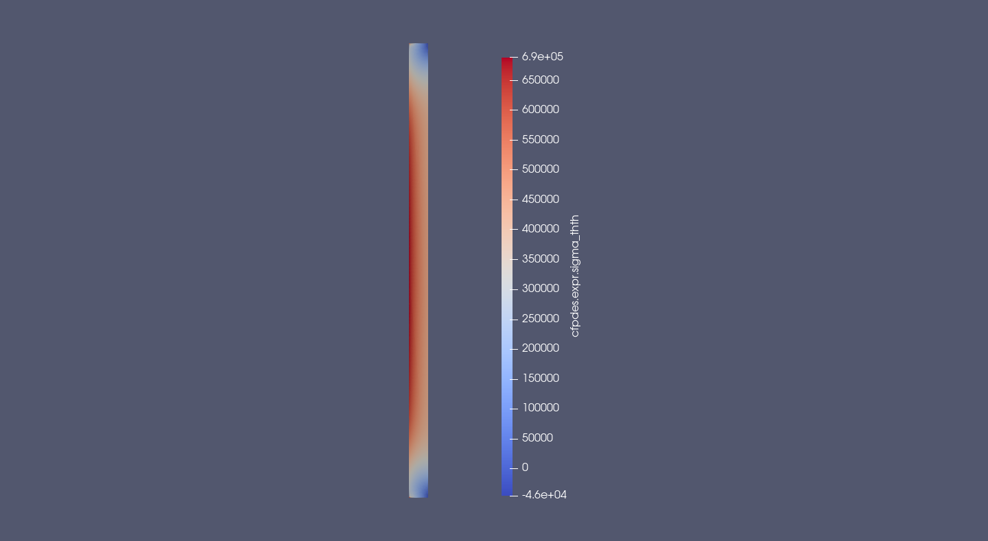
\(\scriptsize{\bar{\bar{\sigma}}_{\theta \theta} = \frac{\lambda + 2\mu}{r} \, u_r + \lambda \, \frac{\partial u_r}{\partial r} + \lambda \, \frac{\partial u_z}{\partial z}- (3\lambda + 2\mu) \, \alpha_T \, \left(T-T_0\right) (Pa)}\)

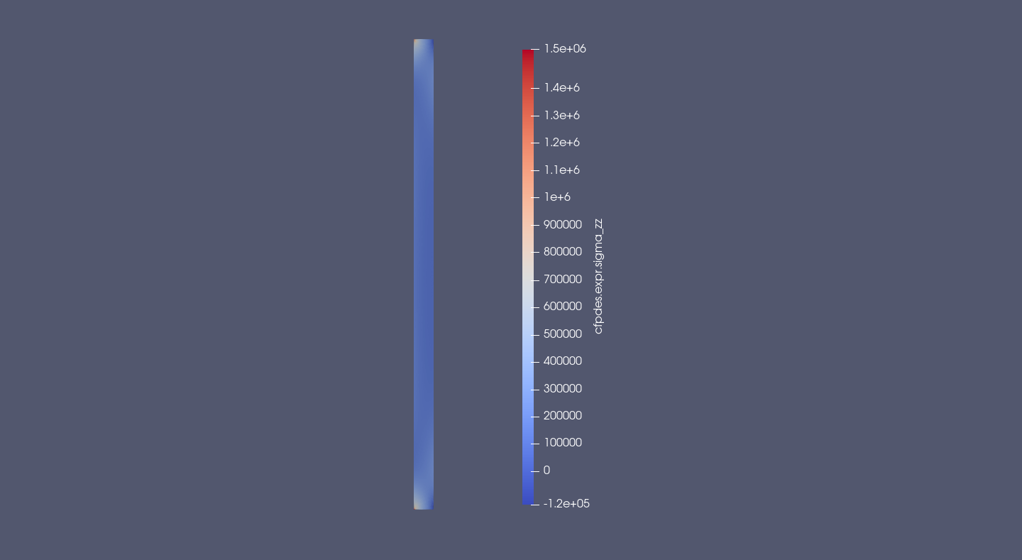
\(\scriptsize{\bar{\bar{\sigma}}_{zz} = \frac{\lambda}{r} \, u_r + \lambda \, \frac{\partial u_r}{\partial r} + \left( \lambda + 2\mu \right) \, \frac{\partial u_z}{\partial z} - (3\lambda + 2\mu) \, \alpha_T \, \left( T-T_0 \right) (Pa)}\)

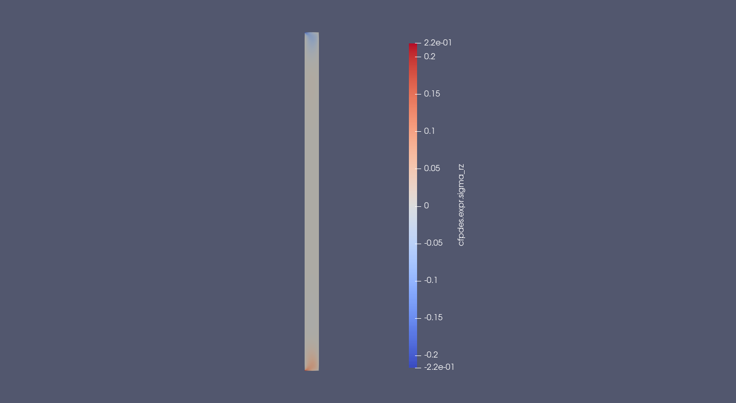
\(\bar{\bar{\sigma}}_{rz} = \mu \, \left( \frac{\partial u_r}{\partial z} + \frac{\partial u_z}{\partial r} \right) (Pa)\)

The radial stress is uniform by the Oz axis and have a form. The minimum is reached around the middle.

The orthoradial stress is the greatest contribution of deformation. The orthoradial stress is uniform by the Oz axis and have a form of an upturned bell. The minimum is reached around the middle.

The z-deformation near of the center is symetric by Oz axis. The cylinder compresses near of the interior and it expands near of the exterior.

The rz-shear is great around the embededding and null in the rest of cylinder.

12.4. Other Tensor

12.4.1. Criterion of Von Mises \(\bar{\bar{\sigma}}_{vm}\)

The tensor of Von Mises permits to say if the matters is in elastic state or not. If the tensor exceeds an matter’s parameter, the matter pass to elastic state to plastic state.

\[\begin{eqnarray*} \bar{\bar{\sigma}}_{Von \, Misses} &=& \sqrt{3 \, J_2} \\ &=& \sqrt{ \frac{13}{2} \, \left( \bar{\bar{\sigma}}_1^2+\bar{\bar{\sigma}}_2^2+\bar{\bar{\sigma}}_3^2-\bar{\bar{\sigma}}_1 \bar{\bar{\sigma}}_2 - \bar{\bar{\sigma}}_1 \bar{\bar{\sigma}}_3 - \bar{\bar{\sigma}}_2 \bar{\bar{\sigma}}_3 \right) } \end{eqnarray*}\]

The \(\sigma_i\) are the principles tensors, the eigenvalues of stress tensor \(\bar{\bar{\sigma}}\).

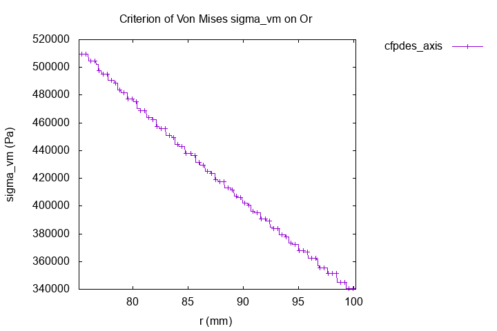
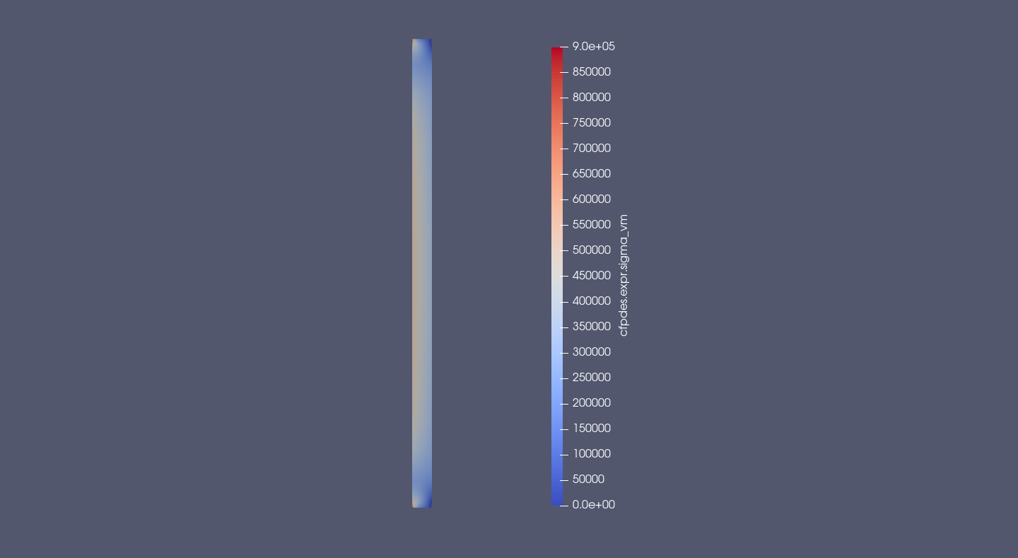
\(\bar{\bar{\sigma}}_{vm} (Pa)\)

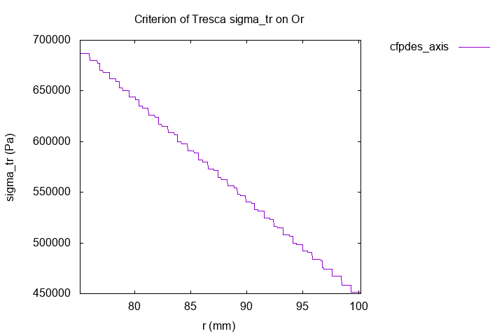
12.4.2. Criterion of Tresca \(\bar{\bar{\sigma}}_{tr}\)

The tensor of Tresca permits to say if the matters is in elastic state or not. If the tensor exceeds an matter’s parameter, the matter pass to elastic state to plastic state.

\[ \bar{\bar{\sigma}}_{tr} = max \left( |\bar{\bar{\sigma}}_1-\bar{\bar{\sigma}}_2|, \, |\bar{\bar{\sigma}}_1-\bar{\bar{\sigma}}_3|, \, |\bar{\bar{\sigma}}_2-\bar{\bar{\sigma}}_3| \right)\]

The \(\sigma_i\) are the principles tensors, the eigenvalues of stress tensor \(\bar{\bar{\sigma}}\).

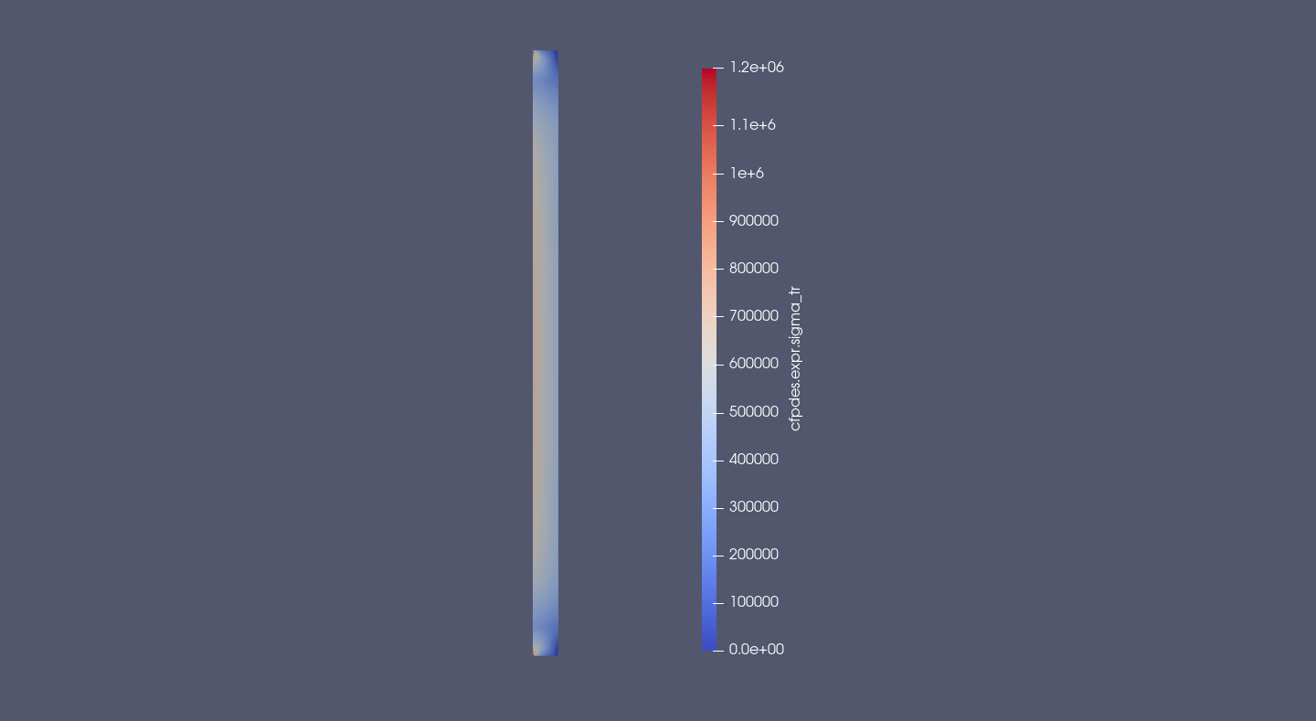
\(\bar{\bar{\sigma}}_{tr} (Pa)\)

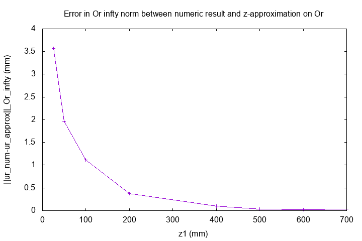
13. Convergence

I do a "convergence study" with error of displacement \(u_r\) on Or axis with analytical approximation solve :

\[\left\{ \begin{eqnarray*} u_{r \, approx}(r) &=& C_1 \, r + \frac{C_2}{r} + u_{pr}(r) \\ u_{pr}(r) &=& - \frac{(1+v)(1-2v)}{E (1-v)}\, J_{int} r_{int} \, \frac{1}{4} \, r ln(\frac{r}{r_{int}}) \left[ B_z(r) + B_z(r_{int}) + \frac{\Delta B_z}{ln(r_{ext}/r_{int})} \right] \\ C_1 &=& \frac{1}{r_{int}^2-r_{ext}^2} \left( r_{ext}^2 \left( (1-v) \frac{\partial u_r}{\partial r}(r_{ext}) + v \frac{u_r(r_{ext})}{r_{ext}} \right) - r_{int}^2 \left( (1-v) \frac{\partial u_r}{\partial r}(r_{int}) + v \frac{u_r(r_{int})}{r_{int}} \right) \right) \\ C_2 &=& \frac{1}{2v-1} \frac{r_{int}^2 r_{ext}^2}{r_{int}^2-r_{ext}^2} \left( (1-v) \frac{\partial u_r}{\partial r}(r_{int}) + v \frac{u_r(r_{int})}{r_{int}} - (1-v) \frac{\partial u_r}{\partial r}(r_{ext}) - v \frac{u_r(r_{ext})}{r_{ext}} \right) \end{eqnarray*} \right.\]

With supposition : the height \(z_1\) is infty.

I compute the error between my numeric result with cfpdes in axisymmetric with different half-height \(z_1\) and the analytical solve with z-approximation with infty norm on Or axis :

\[ ||u_r(z_1) - u_{r \, approx}||_{Or \, \infty} = \underset{r_{int} \leq r \leq r_{ext}}{max} \left| u_r(z_1)(r,0) - u_{r \, approx}(r) \right|\]

Error

Error

The red curves correspond to z-approximation analytical solve (with the half-height \(z_1 = \infty\)).

There are a problem for convergence. The numeric method do not converge in analytical approximation solve for great half-height \(z_1\). But, the numeric method seems converge on limit (greater than the analytical approximation solve).

The error for \(z_1=800 mm\) is equal to \(0.033 mm\). The curve is near than the approximation.

14. Documentation

Solenoid Magnet Design, D. B. Montgomery, Wiley-Interscience, New-York, 1969