Thermo-magnetism problem

This page presents the thermo-magnetism equations in three dimensions and in axisymmetrical coordinates.

1. General Case

For the next calculs, we introduce :

\(\Omega\) the domain, comprising the conductor (or superconductor) domain \(\Omega_c\) and non conducting materials \(\Omega_n\) (\(\mathbf{J} = 0\)) like air. Let \(\Gamma = \partial \Omega\) the bound of \(\Omega\), \(\Gamma_D\) the bound with Dirichlet boundary condition and \(\Gamma_N\) the bound with Neumann boundary condition, such that \(\Gamma = \Gamma_D \cup \Gamma_N\). Let \(\Gamma_c = \partial \Omega_c\) the bound of \(\Omega_c\), \(\Gamma_{Dc}\) the bound with Dirichlet boundary condition and \(\Gamma_{Nc}\) the bound with Neumann boundary condition, such that \(\Gamma_c = \Gamma_{Dc} \cup \Gamma_{Nc}\).

We note \(\mathbf{n}\) the exterior normal of \(\Gamma\) to \(\Omega\).

We solve the A-V Formulation (the equation which govern the electromagnetism in Approximation in Maxwell Quasi Static) coupled with Heat Equation (the equation which governs the temperature) :

\[\left\{ \begin{matrix} \nabla \times \left( \frac{1}{\mu} \nabla \times \textbf{A} \right) + \sigma \frac{\partial \textbf{A}}{\partial t} + \sigma \nabla V &=& 0 & \text{ on } \Omega & \text{(AV-1)} \\ \nabla \cdot \left( \sigma \nabla V + \sigma \frac{\partial \textbf{A}}{\partial t} \right) &=& 0 & \text{ on } \Omega_c & \text{(AV-2)} \\ \mathbf{A} \times \mathbf{n} &=& 0 & \text{ on } \Gamma_D & \text{(AV-D)} \\ \left( \nabla \times \mathbf{A} \right) \times \mathbf{n} &=& 0 & \text{ on } \Gamma_N & \text{(AV-N)} \\ \rho C_p \, \frac{\partial T}{\partial t} - k \Delta T &=& Q & \text{ on } \Omega_c & \text{(Heat)} \\ \frac{\partial T}{\partial \mathbf{n}} &=& 0 & \text{ on } \Gamma_{Nc} & \text{(Heat-N)} \\ - k \, \frac{\partial T}{\partial \mathbf{n}} &=& h \, \left( T - T_c \right) & \text{ on } \Gamma_{Rc} & \text{(Heat-R)} \\ \end{matrix} \right.\]

With :

  • \(\mathbf{A}\) such that \(\mathbf{B} = \nabla \times \mathbf{A}\)

  • \(\rho\) : density \((kg/m^3)\)

  • \(T\) : temperature \((K)\)

  • \(C_p\) : thermal capacity \((J/K/kg)\)

  • \(\sigma\) : electric conductivity \((S/m)\)

  • \(k\) : thermal conductivity \((W/m/K)\)

  • \(\mu\) : electric permeability \((kg/A^2/S^2)\)

  • \(Q\) : source term \((K)\)

The Heat Equation will resolved on conductor \(\Omega_c\).

The Joules effect gives us the thermal source term :

\[ Q = \mathbf{J} \cdot \mathbf{E}\]

With \(\mathbf{J}\) the current and \(\mathbf{E}\) the electric field.

Or we know with section A-V Formulation, \(\mathbf{E} = -\nabla V - \frac{\partial \mathbf{A}}{\partial t}\) and \(\mathbf{J} = \sigma \, \mathbf{E}\). Thus :

\[Q = \sigma \left( \nabla V + \frac{\partial \mathbf{A}}{\partial t} \right) \cdot \left( \nabla V + \frac{\partial \mathbf{A}}{\partial t} \right)\]

We obtain :

Differential Formulation
\[\small{ \left\{ \begin{matrix} \nabla \times \left( \frac{1}{\mu} \nabla \times \textbf{A} \right) + \sigma \frac{\partial \textbf{A}}{\partial t} + \sigma \nabla V &=& 0 & \text{ on } \Omega & \text{(AV-1)} \\ \nabla \cdot \left( \sigma \nabla V + \sigma \frac{\partial \textbf{A}}{\partial t} \right) &=& 0 & \text{ on } \Omega_c & \text{(AV-2)} \\ \mathbf{A} \times \mathbf{n} &=& 0 & \text{ on } \Gamma_D & \text{(D)} \\ \left( \nabla \times \mathbf{A} \right) \times \mathbf{n} &=& 0 & \text{ on } \Gamma_N & \text{(N)} \\ \rho C_p \, \frac{\partial T}{\partial t} - k \Delta T &=& \sigma \left( \nabla V + \frac{\partial \mathbf{A}}{\partial t} \right) \cdot \left( \nabla V + \frac{\partial \mathbf{A}}{\partial t} \right) & \text{ on } \Omega_c & \text{(Heat)} \\ \frac{\partial T}{\partial \mathbf{n}} &=& 0 & \text{ on } \Gamma_{Nc} & \text{(Heat-N)} \\ - k \, \frac{\partial T}{\partial \mathbf{n}} &=& h \, \left( T - T_c \right) & \text{ on } \Gamma_{Rc} & \text{(Heat-R)} \\ \end{matrix} \right. }\]

We can summer the coupling by this diagram :

diagram physics 2
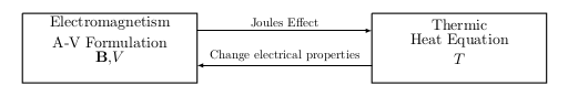
Diagram of Coupling problem

2. With Gauge condition

Like on page MQS + gauge condition, we can add Gauge condiction on magnetic potential field :

\[ \nabla \cdot \mathbf{A} = 0\]

It give new equations :

Coupled A-V Formulation with gauge condition and Heat Equation
\[\text{(AV+gauge)} \left\{ \begin{matrix} \frac{1}{\mu} \Delta \textbf{A} + \sigma \frac{\partial \textbf{A}}{\partial t} &=& - \sigma \nabla V & \text{ on } \Omega & \text{(AV+gauge-1)} \\ \nabla \cdot \left( \sigma \nabla V \right) &=& - \nabla \cdot \left( \sigma \frac{\partial \mathbf{A}}{\partial t} \right) & \text{ on } \Omega_c & \text{(AV-2)} \\ \mathbf{A} &=& 0 & \text{ on } \Gamma_D & \text{(DA)} \\ \frac{\partial \mathbf{A}}{\partial \mathbf{n}} &=& 0 & \text{ on } \Gamma_N & \text{(NA)} \\ V &=& V_0 & \text{ on } \Gamma_{DV} & \text{(DV)} \\ \frac{\partial V}{\partial \mathbf{n}} &=& 0 & \text{ on } \Gamma_{NV} & \text{(NV)} \\ \rho C_p \, \frac{\partial T}{\partial t} - k \Delta T &=& \sigma \left( \nabla V + \frac{\partial \mathbf{A}}{\partial t} \right) \cdot \left( \nabla V + \frac{\partial \mathbf{A}}{\partial t} \right) & \text{ on } \Omega_c & \text{(Heat)} \\ \frac{\partial T}{\partial \mathbf{n}} &=& 0 & \text{ on } \Gamma_{Nc} & \text{(Heat-N)} \\ - k \, \frac{\partial T}{\partial \mathbf{n}} &=& h \, \left( T - T_c \right) & \text{ on } \Gamma_{Rc} & \text{(Heat-R)} \\ \end{matrix} \right.\]
The interest of thise fomulation is to remove the rotationals to implement on CFPDEs. CFPDEs doesn’t implement rotationals.

3. Axisymmetric case

In this subsection, we express the Coupled Equation on geometry in axisymmetric.

On equations A-V Formulation, we suppose the geometry, the parameters, \(B\), \(T\) are independent by \(\theta\) (of cylindric coordinates \((r,\theta,z)\)) and we suppose \(V\) uniquely dependant by \(\theta\) and know (\(V=\frac{U}{2\pi} \, \theta\)).

We note \(\Omega^{axis}\) (respectively \(\Omega^{axis}_c\), \(\Gamma^{axis}\), \(\Gamma_D^{axis}\), \(\Gamma_N^{axis}\), \(\Gamma_c^{axis}\), \(\Gamma_{Nc}^{axis}\) and \(\Gamma_{Rc}^{axis}\)) the representation of \(\Omega\) (respectively \(\Omega_c\), \(\Gamma\), \(\Gamma_D\), \(\Gamma_N\), \(\Gamma_c\), \(\Gamma_{Nc}\) and \(\Gamma_{Rc}\)) in axisymmetric coordinates.

We note \(u = \begin{pmatrix} u_r \\ u_{\theta} \\ u_z \end{pmatrix}_{cyl}\) the coordinates of \(u \in \mathbb{R}^3\) in cylindrical base.

We note \(\mathbf{n}^{axis} = \begin{pmatrix} n^{axis}_r \\ n^{axis}_z \end{pmatrix}_{cyl}\) the exterior normal of \(\Gamma^{axis}\) on \(\Omega^{axis}\).

We obtain reduce of coponent of magnetic potential field :

\[ \mathbf{A} = \begin{pmatrix} 0 \\ A_{\theta} \\ 0 \end{pmatrix}_{cyl}\]

The detail of calcul do here :

We assume that \(V\) is known : \(V = \frac{U}{2\pi} \, \theta\) with \(U\) tension.

Differential Formulation in Axisymmetric
\[\text{(AV+Heat Axis)} \left\{ \begin{matrix} \sigma \frac{\partial \Phi}{\partial t} - \frac{1}{\mu} \Delta \Phi + \frac{2}{\mu \, r} \frac{\partial \Phi}{\partial r} + \sigma \frac{\partial V}{\partial \theta} = 0 & \text{ on } \Omega & \text{(AV-1 Axis)} \\ V = \frac{U}{2\pi} \, \theta & \text{ on } \Omega_c^{axis} & \text{(AV-2 Axis)} \\ A_{\theta} = 0 & \text{ on } \Gamma_D^{axis} & \text{(D Axis)} \\ \frac{\partial A_{\theta}}{\partial \mathbf{n}^{axis}} = 0 & \text{ on } \Gamma_N^{axis} & \text{(N Axis)} \\ \rho C_p \, \frac{\partial T}{\partial t} - k \Delta T = \sigma \, \left( \frac{1}{r} \, \frac{\partial V}{\partial \theta} + \frac{\partial A_{\theta}}{\partial t} \right)^2 & \text{ on } \Omega_c^{axis} & \text{(Heat Axis)} \\ \frac{\partial T}{\partial \mathbf{n}^{axis}} = 0 & \text{ on } \Gamma_{Nc}^{axis} & \text{(Nc Axis)} \\ - k \, \frac{\partial T}{\partial \mathbf{n}^{axis}} = h \, \left( T - T_c \right) & \text{ on } \Gamma_{Rc}^{axis} & \text{(Rc Axis)} \end{matrix} \right.\]
  • With \(\Phi = r \, A_{\theta}\)