Equations of Elasticity in Static Case

This section presents the equation of elasticity in stationary case and axisymetric case.

1. In General Case

1.1. Differential Formulation

We search the displacement \(\mathbf{u} \in \mathbb{R}^3\) induced by a transformation. The domain of resolution is \(\Omega_c\) with bounds \(\Gamma_c\), \(\Gamma_{D \hspace{0.05cm} elas}\) the bound of Dirichlet conditions, \(\Gamma_{N \hspace{0.05cm} elas}\) the bound of Neumann conditions and \(\Gamma_{R \hspace{0.05cm} elas}\) the bound of Robin conditions such that \(\Gamma_{D \hspace{0.05cm} elas} \cup \Gamma_{N \hspace{0.05cm} elas} \cup \Gamma_{R \hspace{0.05cm} elas} = \Gamma_c\).

We introduce the Lamé’s coefficients :

\[\lambda = \frac{E \, \nu}{(1-2 v) \, (1+\nu)}, \ \mu = \frac{E}{2 \, (1+\nu)}\]

With :

Young modulus \(E\), it represents the rigidity of materials (\(10^5 \leq \lambda \leq 10^{10}\))
Poisson’s coefficient \(\nu\), it represents the incompressibility of materials (\(0 \leq \mu \leq 0.5\)). If \(\mu = 0.5\), the materials is perfectly incompressible.

Conversely :

\[ \nu = \frac{\lambda}{2 (\lambda + \mu)}, E = \frac{\mu (3\lambda + 2\mu)}{\lambda + \mu}\]

We introduce the tensor of small deformations :

\[ \bar{\bar{\epsilon}}_{ij} = \frac{1}{2} \, \left( \frac{\partial u_{j}}{\partial j} + \frac{\partial u_{i}}{\partial i} \right) \ \text{ for } i,j = x, y, z\]

And, the stress tensor :

\[ \bar{\bar{\sigma}} = C \, \bar{\bar{\epsilon}}\]

With \(C\), a law which determenized by material.

The equilibrium equations with boundary conditions of Dirichlet, Neumann and Robin is written like :

Differential Formulation of Elasticity Equation in Stationary Case

\[\text{(Static Elasticity)} \left\{ \begin{matrix} - \nabla \cdot \bar{\bar{\sigma}} = \mathbf{F} & \text{on } \Omega_c & \text{(Static Elas-1)} \\ \mathbf{u} = \mathbf{u_0} & \text{on } \Gamma_{D \hspace{0.05cm} elas} & \text{(D elas)} \\ \bar{\bar{\sigma}} \cdot \mathbf{n} = g_N & \text{on } \Gamma_{N \hspace{0.05cm} elas} & \text{(N elas)} \\ \bar{\bar{\sigma}} \cdot \mathbf{n} + k \, \mathbf{u} = g_R & \text{on } \Gamma_{R \hspace{0.05cm} elas} & \text{(R elas)} \end{matrix} \right.\]

With :

Displacement \(\mathbf{u} = \begin{pmatrix} u_x \\ u_y \\ u_z \end{pmatrix}\)
Stress Tensor : \(\bar{\bar{\sigma}}\)
Stiffness tensor : \(k\)
Volumic Forces : \(\mathbf{F}\)

And notations :

Divergence of tensor : \(\nabla \cdot \bar{\bar{\sigma}} = \begin{pmatrix} \nabla \cdot \bar{\bar{\sigma}}_{x,:} \\ \nabla \cdot \bar{\bar{\sigma}}_{y,:} \\ \nabla \cdot \bar{\bar{\sigma}}_{z,:} \end{pmatrix} = \begin{pmatrix} \frac{\partial \bar{\bar{\sigma}}_{xx}}{\partial x} + \frac{\partial \bar{\bar{\sigma}}_{xy}}{\partial y} + \frac{\partial \bar{\bar{\sigma}}_{xz}}{\partial z} \\ \frac{\partial \bar{\bar{\sigma}}_{yx}}{\partial x} + \frac{\partial \bar{\bar{\sigma}}_{yy}}{\partial y} + \frac{\partial \bar{\bar{\sigma}}_{yz}}{\partial z} \\ \frac{\partial \bar{\bar{\sigma}}_{zx}}{\partial x} + \frac{\partial \bar{\bar{\sigma}}_{zy}}{\partial y} + \frac{\partial \bar{\bar{\sigma}}_{zz}}{\partial z} \end{pmatrix}\)
Scalar produce of tensor : \(\bar{\bar{\sigma}} \cdot \mathbf{n} = \begin{pmatrix} \bar{\bar{\sigma}}_{x,:} \cdot \mathbf{n} \\ \bar{\bar{\sigma}}_{y,:} \cdot \mathbf{n} \\ \bar{\bar{\sigma}}_{z,:} \cdot \mathbf{n} \end{pmatrix} = \begin{pmatrix} \bar{\bar{\sigma}}_{xx} \, n_x + \bar{\bar{\sigma}}_{xy} \, n_y + \bar{\bar{\sigma}}_{xz} \, n_z \\ \bar{\bar{\sigma}}_{yx} \, n_x + \bar{\bar{\sigma}}_{yy} \, n_y + \bar{\bar{\sigma}}_{yz} \, n_z \\ \bar{\bar{\sigma}}_{zx} \, n_x + \bar{\bar{\sigma}}_{zy} \, n_y + \bar{\bar{\sigma}}_{zz} \, n_z \end{pmatrix}\)

In the rest of this section, we use the Hooke law :

\[ \bar{\bar{\sigma}}^E = \lambda \, Tr(\bar{\bar{\epsilon}}) \, Id + 2 \, \mu \, \bar{\bar{\epsilon}}\]

It can rewrite like :

\[ \bar{\bar{\sigma}}_{ij}^E = \lambda \, \delta_{ij} \, \nabla \cdot \mathbf{u} + 2 \, \mu \, \bar{\bar{\epsilon}}_{ij}\]

And the Thermal Dilatation law :

\[ \bar{\bar{\sigma}}^T = - (3 \lambda + 2 \mu) \, \alpha_T \, \left( T - T_0 \right) \, Id\]

With linear dilatation coefficient \(\alpha_T\), \(T\) the temperature and \(T_0\) the temperature of reference (or rest temperature).

Thus, the stress tensor is writen like :

\[\begin{eqnarray*} \bar{\bar{\sigma}} &=& \bar{\bar{\sigma}}^E + \bar{\bar{\sigma}}^T \\ &=& \lambda \, Tr(\bar{\bar{\epsilon}}) \, Id + 2 \, \mu \, \bar{\bar{\epsilon}} - (3 \lambda + 2 \mu) \, \alpha_T \, \left( T - T_0 \right) \, Id \end{eqnarray*}\]

Or :

\[ \bar{\bar{\sigma}}_{ij} = \lambda \, \delta_{ij} \, \nabla \cdot \mathbf{u} + 2 \, \mu \, \bar{\bar{\epsilon}}_{ij} - (3 \lambda + 2 \mu) \, \delta_{ij} \, \alpha_T \, \left( T - T_0 \right)\]

1.2. Weak Formulation

We express the weak formulation of (Static Elasticity) component by component.

We will here deal only with strong Dirichlet conditions (on \(\Gamma_{D \hspace{0.05cm} elas}\)) that is why the function space is set to \(H^1_{u_0}(\Omega) = \{ u \in H^1(\Omega), \ u = u_0 \text{ on } \Gamma_{D \hspace{0.05cm} elas} \}\).

By multiplying the x component of (Static Elas-1) by \(\xi_x\) of \(\mathbf{ξ} = \begin{pmatrix} \xi_x \\ \xi_y \\ \xi_z \end{pmatrix} \in H^1_{u_0}(\Omega)\) and integrating over \(\Omega_c\), we obtain :

\[ - \int_{\Omega_c}{\left( \frac{\partial \bar{\bar{\sigma}}_{xx}}{\partial x} + \frac{\partial \bar{\bar{\sigma}}_{xy}}{\partial y} + \frac{\partial \bar{\bar{\sigma}}_{xz}}{\partial z} \right) \, \xi_x } = \int_{\Omega_c}{ F_x \, \xi_x }\]

By the Formula of Green (First Form) :

\[ \int_{\Omega_c}{ \bar{\bar{\sigma}}_{xx} \, \frac{\partial \xi_x}{\partial x} + \bar{\bar{\sigma}}_{xy} \, \frac{\partial \xi_x}{\partial y} + \bar{\bar{\sigma}}_{xz} \, \frac{\partial \xi_x}{\partial z} } - \int_{\Gamma_c}{ \bar{\bar{\sigma}}_{xx} \, \xi_x \, n_x + \bar{\bar{\sigma}}_{xy} \, \xi_x \, n_y + \bar{\bar{\sigma}}_{xz} \, \xi_x \, n_z } = \int_{\Omega_c}{ F_x \, \xi_x }\]

With notations :

\[ \int_{\Omega_c}{ \bar{\bar{\sigma}}_{xx} \, \frac{\partial \xi_x}{\partial x} + \bar{\bar{\sigma}}_{xy} \, \frac{\partial \xi_x}{\partial y} + \bar{\bar{\sigma}}_{xz} \, \frac{\partial \xi_x}{\partial z} } - \int_{\Gamma_c}{ \left( \bar{\bar{\sigma}}_{x,:} \cdot \mathbf{n} \right) \, \xi_x } = \int_{\Omega_c}{ F_x \, \xi_x }\]

We apply the boundary conditions :

\[ \int_{\Omega_c}{ \bar{\bar{\sigma}}_{xx} \, \frac{\partial \xi_x}{\partial x} + \bar{\bar{\sigma}}_{xy} \, \frac{\partial \xi_x}{\partial y} + \bar{\bar{\sigma}}_{xz} \, \frac{\partial \xi_x}{\partial z} } - \int_{\Gamma_{N \hspace{0.05cm} elas}}{ g_{Nx} \, \xi_x } - \int_{\Gamma_{R \hspace{0.05cm} elas}}{ \left( g_{Rx} - \left( k \, u \right)_x \right) \, \xi_x } = \int_{\Omega_c}{ F_x \, \xi_x }\]

\[ \int_{\Omega_c}{ \bar{\bar{\sigma}}_{xx} \, \frac{\partial \xi_x}{\partial x} + \bar{\bar{\sigma}}_{xy} \, \frac{\partial \xi_x}{\partial y} + \bar{\bar{\sigma}}_{xz} \, \frac{\partial \xi_x}{\partial z} } = \int_{\Omega_c}{ F_x \, \xi_x } + \int_{\Gamma_{N \hspace{0.05cm} elas}}{ g_{Nx} \, \xi_x } + \int_{\Gamma_{R \hspace{0.05cm} elas}}{ \left( g_{Rx} - \left( k \, u \right)_x \right) \, \xi_x }\]

We do the same with \(y\) and \(z\) components and we obtain the weak formulation of (Static Elasticity) component by component :

Weak Formulation of Elasticity Equation in Stationnary Case Component by Component

\[\text{(Weak Static Elasticity Component by Component)} \\ \left\{ \begin{matrix} \int_{\Omega_c}{ \bar{\bar{\sigma}}_{xx} \, \frac{\partial \xi_x}{\partial x} + \bar{\bar{\sigma}}_{xy} \, \frac{\partial \xi_x}{\partial y} + \bar{\bar{\sigma}}_{xz} \, \frac{\partial \xi_x}{\partial z} } = \int_{\Omega_c}{ F_x \, \xi_x } + \int_{\Gamma_{N \hspace{0.05cm} elas}}{ g_{Nx} \, \xi_x } + \int_{\Gamma_{R \hspace{0.05cm} elas}}{ \left( g_{Rx} - \left( k \, u \right)_x \right) \, \xi_x } \\ \int_{\Omega_c}{ \bar{\bar{\sigma}}_{yx} \, \frac{\partial \xi_y}{\partial x} + \bar{\bar{\sigma}}_{yy} \, \frac{\partial \xi_y}{\partial y} + \bar{\bar{\sigma}}_{yz} \, \frac{\partial \xi_y}{\partial z} } = \int_{\Omega_c}{ F_y \, \xi_y } + \int_{\Gamma_{N \hspace{0.05cm} elas}}{ g_{Ny} \, \xi_y } + \int_{\Gamma_{R \hspace{0.05cm} elas}}{ \left( g_{Ry} - \left( k \, u \right)_y \right) \, \xi_y } \\ \int_{\Omega_c}{ \bar{\bar{\sigma}}_{zx} \, \frac{\partial \xi_z}{\partial x} + \bar{\bar{\sigma}}_{zy} \, \frac{\partial \xi_z}{\partial y} + \bar{\bar{\sigma}}_{zz} \, \frac{\partial \xi_z}{\partial z} } = \int_{\Omega_c}{ F_z \, \xi_z } + \int_{\Gamma_{N \hspace{0.05cm} elas}}{ g_{Nz} \, \xi_z } + \int_{\Gamma_{R \hspace{0.05cm} elas}}{ \left( g_{Rz} - \left( k \, u \right)_z \right) \, \xi_z } \\ \text{for } \mathbf{ξ} = \begin{pmatrix} \xi_x \\ \xi_y \\ \xi_z \end{pmatrix} \in H^1_{u_0}(\Omega_c) \end{matrix} \right.\]

To obtain the vectorial form, we sum the three equations :

Weak Formulation of Elasticity Equation in Stationnary Case Vectorial

\[\text{(Weak Static Elasticity Vectorial)} \\ \left\{ \begin{matrix} \int_{\Omega_c}{ \bar{\bar{\sigma}}_{xx} \, \frac{\partial \xi_x}{\partial x} + \bar{\bar{\sigma}}_{xy} \, \frac{\partial \xi_x}{\partial y} + \bar{\bar{\sigma}}_{xz} \, \frac{\partial \xi_x}{\partial z} + \bar{\bar{\sigma}}_{yx} \, \frac{\partial \xi_y}{\partial x} + \bar{\bar{\sigma}}_{yy} \, \frac{\partial \xi_y}{\partial y} + \bar{\bar{\sigma}}_{yz} \, \frac{\partial \xi_y}{\partial z} + \bar{\bar{\sigma}}_{zx} \, \frac{\partial \xi_z}{\partial x} + \bar{\bar{\sigma}}_{zy} \, \frac{\partial \xi_z}{\partial y} + \bar{\bar{\sigma}}_{zz} \, \frac{\partial \xi_z}{\partial z} } = \int_{\Omega_c}{ \mathbf{F} \cdot \mathbf{ξ} } + \int_{\Gamma_{N \hspace{0.05cm} elas}}{ \mathbf{g_N} \cdot \mathbf{ξ} } + \int_{\Gamma_{R \hspace{0.05cm} elas}}{ \left( \mathbf{g_R} - ku \right) \cdot \mathbf{ξ} } \\ \text{for } \mathbf{ξ} = \begin{pmatrix} \xi_x \\ \xi_y \\ \xi_z \end{pmatrix} \in H^1_{u_0}(\Omega_c) \end{matrix} \right.\]

2. In axisymmetric coordinates

2.1. Differential Formulation

On equations (Static Elasticity), we suppose the geometry and the parameters are independent by \(\theta\) (of cylindric coordinates \((r,\theta,z)\)).

We note \(\Omega^{axis}_c\) (respectively \(\Gamma_c^{axis}\), \(\Gamma_{D \hspace{0.05cm} elas}^{axis}\), \(\Gamma_{N \hspace{0.05cm} elas}^{axis}\) and \(\Gamma_{R \hspace{0.05cm} elas}^{axis}\)) the representation of \(\Omega_c\) (respectively \(\Gamma_c\), \(\Gamma_{D \hspace{0.05cm} elas}\), \(\Gamma_{N \hspace{0.05cm} elas}\)) and \(\Gamma_{R \hspace{0.05cm} elas}\) in axisymmetric coordinates.

We note \(\mathbf{u} = \begin{pmatrix} u_r \\ u_{\theta} \\ u_z \end{pmatrix}_{cyl}\) the coordinates of \(u \in \mathbb{R}^3\) in cylindrical base and by abuse of language, \(\mathbf{u} = \begin{pmatrix} u_r \\ u_z \end{pmatrix}_{axis}\) the coordinates of \(u \in \mathbb{R}^3\) in axisymmetrical base.

We note \(\mathbf{n}^{axis} = \begin{pmatrix} n^{axis}_r \\ n^{axis}_z \end{pmatrix}_{axis}\) the exterior normal of \(\Gamma^{axis}\) on \(\Omega^{axis}\).

The tensor of small deformations becomes :

\[\begin{align*} \bar{\bar{\epsilon}}_{rr} &= \frac{\partial u_r}{\partial r} , & \bar{\bar{\epsilon}}_{rz} &= \frac{1}{2} \left( \frac{\partial u_z}{\partial r} + \frac{\partial u_r}{\partial z} \right) \\ \bar{\bar{\epsilon}}_{zz} &= \frac{\partial u_z}{\partial z} , & \bar{\bar{\epsilon}}_{r\theta} &= 0 \\ \bar{\bar{\epsilon}}_{\theta \theta} &= \frac{1}{r} \, u_r , & \bar{\bar{\epsilon}}_{\theta z} &= 0 \end{align*}\]

And the stress tensor :

\[\begin{align*} \bar{\bar{\sigma}}_{rr} &= \frac{\lambda}{r} \, u_r + \left( \lambda + 2\mu \right) \, \frac{\partial u_r}{\partial r} + \lambda \, \frac{\partial u_z}{\partial z} - (3\lambda + 2 \mu) \, \alpha_T \, \left( T-T_0 \right) , & \bar{\bar{\sigma}}_{rz} &= \mu \, \left( \frac{\partial u_r}{\partial z} + \frac{\partial u_z}{\partial r} \right) \\ \bar{\bar{\sigma}}_{zz} &= \frac{\lambda}{r} \, u_r + \lambda \, \frac{\partial u_r}{\partial r} + \left( \lambda + 2\mu \right) \, \frac{\partial u_z}{\partial z} - (3\lambda + 2 \mu) \, \alpha_T \, \left( T-T_0 \right) , & \bar{\bar{\sigma}}_{r \theta} &= 0 \\ \bar{\bar{\sigma}}_{\theta \theta} &= \frac{\lambda + 2\mu}{r} \, u_r + \lambda \, \frac{\partial u_r}{\partial r} + \lambda \, \frac{\partial u_z}{\partial z} - (3\lambda + 2 \mu) \, \alpha_T \, \left( T-T_0 \right), & \bar{\bar{\sigma}}_{z \theta} &= 0 \end{align*}\]

We have in cylindrical coodinates :

\[\begin{eqnarray*} \nabla \cdot \bar{\bar{\sigma}} &=& \begin{pmatrix} \frac{\partial \bar{\bar{\sigma}}_{rr}}{\partial r} + \frac{1}{r} \frac{\partial \bar{\bar{\sigma}}_{r\theta}}{\partial \theta} + \frac{\partial \bar{\bar{\sigma}}_{rz}}{\partial z} + \frac{\bar{\bar{\sigma}}_{rr} - \bar{\bar{\sigma}}_{\theta \theta}}{r} \\ \frac{\partial \bar{\bar{\sigma}}_{\theta r}}{\partial r} + \frac{1}{r} \frac{\partial \bar{\bar{\sigma}}_{\theta \theta}}{\partial \theta} + \frac{\partial \bar{\bar{\sigma}}_{zz}}{\partial z} + \frac{\bar{\bar{\sigma}}_{r\theta} + \bar{\bar{\sigma}}_{\theta r}}{r} \\ \frac{\partial \bar{\bar{\sigma}}_{zr}}{\partial r} + \frac{1}{r} \frac{\partial \bar{\bar{\sigma}}_{z \theta}}{\partial \theta} + \frac{\partial \bar{\bar{\sigma}}_{zz}}{\partial z} + \frac{\bar{\bar{\sigma}}_{zr}}{r} \end{pmatrix}_{cyl} \\ &=& \begin{pmatrix} \frac{\partial \bar{\bar{\sigma}}_{rr}}{\partial r} + \frac{1}{r} \times 0 + \frac{\partial \bar{\bar{\sigma}}_{rz}}{\partial z} + \frac{\bar{\bar{\sigma}}_{rr} - \bar{\bar{\sigma}}_{\theta \theta}}{r} \\ 0 \, + \, 0 \, + \, 0 \, + \frac{0 + 0}{r} \\ \frac{\partial \bar{\bar{\sigma}}_{rz}}{\partial r} + \frac{1}{r} \times 0 + \frac{\partial \bar{\bar{\sigma}}_{zz}}{\partial z} + \frac{\bar{\bar{\sigma}}_{rz}}{r} \end{pmatrix}_{cyl} \\ &=& \begin{pmatrix} \frac{\partial \bar{\bar{\sigma}}_{rr}}{\partial r} + \frac{\partial \bar{\bar{\sigma}}_{rz}}{\partial z} + \frac{\bar{\bar{\sigma}}_{rr} - \bar{\bar{\sigma}}_{\theta \theta}}{r} \\ 0 \\ \frac{\partial \bar{\bar{\sigma}}_{rz}}{\partial r} + \frac{\partial \bar{\bar{\sigma}}_{zz}}{\partial z} + \frac{\bar{\bar{\sigma}}_{rz}}{r} \end{pmatrix}_{cyl} \end{eqnarray*}\]

We do a rating abuse :

\[ \nabla \cdot \bar{\bar{\sigma}} = \begin{pmatrix} \frac{\partial \bar{\bar{\sigma}}_{rr}}{\partial r} + \frac{\partial \bar{\bar{\sigma}}_{rz}}{\partial z} + \frac{\bar{\bar{\sigma}}_{rr} - \bar{\bar{\sigma}}_{\theta \theta}}{r} \\ \frac{\partial \bar{\bar{\sigma}}_{rz}}{\partial r} + \frac{\partial \bar{\bar{\sigma}}_{zz}}{\partial z} + \frac{\bar{\bar{\sigma}}_{rz}}{r} \end{pmatrix}_{axis}\]

Or, in the other form :

\[ \nabla \cdot \bar{\bar{\sigma}} = \begin{pmatrix} \nabla \cdot \bar{\bar{\sigma}}_{r,:} + \frac{\bar{\bar{\sigma}}_{rr} - \bar{\bar{\sigma}}_{\theta \theta}}{r} \\ \nabla \cdot \bar{\bar{\sigma}}_{z,:} + \frac{\bar{\bar{\sigma}}_{rz}}{r} \end{pmatrix}_{axis}\]

With \(\bar{\bar{\sigma}}_{r,:} = \begin{pmatrix} \bar{\bar{\sigma}}_{rr} & \bar{\bar{\sigma}}_{rz} \end{pmatrix}\) and \(\bar{\bar{\sigma}}_{z,:} = \begin{pmatrix} \bar{\bar{\sigma}}_{rz} & \bar{\bar{\sigma}}_{zz} \end{pmatrix}\)

Differential Formulation of Elasticity Equation in Stationary Case in Axisymmetric

\[\text{(Static Elasticity Axis)} \left\{ \begin{matrix} - \nabla \cdot \bar{\bar{\sigma}} = F & \text{on } \Omega_c^{axis} & \\ \mathbf{u} = 0 & \text{on } \Gamma_{D \hspace{0.05cm} elas}^{axis} & \text{(D axis elas)} \\ \bar{\bar{\sigma}} \cdot \mathbf{n}^{axis} = g_N & \text{on } \Gamma_{N \hspace{0.05cm} elas}^{axis} & \text{(N axis elas)} \\ \bar{\bar{\sigma}} \cdot \mathbf{n}^{axis} + k \, \mathbf{u} = g_R & \text{on } \Gamma_{R \hspace{0.05cm} elas}^{axis} & \text{(R axis elas)} \end{matrix} \right.\]

With : \(\nabla \cdot \bar{\bar{\sigma}} = \begin{pmatrix} \nabla \cdot \bar{\bar{\sigma}}_{r,:} + \frac{\bar{\bar{\sigma}}_{rr} - \bar{\bar{\sigma}}_{\theta \theta}}{r} \\ \nabla \cdot \bar{\bar{\sigma}}_{z,:} + \frac{\bar{\bar{\sigma}}_{rz}}{r} \end{pmatrix}_{axis}\)

2.2. Weak Formulation

This section follows the calculus of book Theorical Physics Reference.

To obtain the weak formulation of axisymetric elastic equation, we pass by the weak formulation of elastic problem in cartesian (Weak Static Elasticity).

We have the formula of changement to cartesian to cylindric :

\[\begin{eqnarray*} u_x &=& cos \theta \, u_r \\ u_y &=& sin \theta \, u_r \\ u_z &=& u_z \end{eqnarray*}\]

\[\begin{eqnarray*} \frac{\partial u_x}{\partial x} &=& \frac{\partial u_r}{\partial r} cos^2 \theta + \frac{1}{r} u_r sin^2 \theta \\ \frac{\partial u_x}{\partial y} &=& \frac{\partial u_r}{\partial r} cos \theta sin \theta + \frac{1}{r} u_r cos \theta sin \theta \\ \frac{\partial u_x}{\partial z} &=& \frac{\partial u_z}{\partial z} cos \theta \end{eqnarray*}\]

\[\begin{eqnarray*} \frac{\partial u_y}{\partial x} &=& \frac{\partial u_r}{\partial r} cos \theta sin \theta + \frac{1}{r} u_r cos \theta sin \theta \\ \frac{\partial u_y}{\partial y} &=& \frac{\partial u_r}{\partial r} sin^2 \theta + \frac{1}{r} u_r cos^2 \theta \\ \frac{\partial u_y}{\partial z} &=& \frac{\partial u_z}{\partial z} sin \theta \end{eqnarray*}\]

\[\begin{eqnarray*} \frac{\partial u_z}{\partial x} &=& \frac{\partial u_z}{\partial z} cos \theta \\ \frac{\partial u_z}{\partial y} &=& \frac{\partial u_z}{\partial z} sin \theta \\ \frac{\partial u_z}{\partial z} &=& \frac{\partial u_x}{\partial z} \end{eqnarray*}\]

The x component of (Weak Static Elasticity) becomes :

\[\scriptsize{ \begin{eqnarray*} \int_{\Omega_c} r \left[ \lambda \left( \frac{\partial u_r}{\partial r} + \frac{1}{r} u_r + \frac{\partial u_z}{\partial z} \right) + 2\mu \left( \frac{\partial u_r}{\partial r} cos^2 \theta + \frac{1}{r} u_r sin^2 \theta \right) - (3\lambda + 2 \mu) \, \alpha_T \, \left( T-T_0 \right) \right] \left( \frac{\partial \xi_r}{\partial r} cos^2 \theta + \frac{1}{r} \xi_r sin^2 \theta \right) + r 2\mu \left( \frac{\partial u_r}{\partial r} cos \theta sin \theta - \frac{1}{r} u_r cos \theta sin \theta \right) \left( \frac{\partial \xi_r}{\partial r} cos \theta sin \theta - \frac{1}{r} \xi_r cos \theta sin \theta \right) \\ \left. + r\mu \left( \frac{\partial u_r}{\partial z} cos \theta + \frac{\partial u_z}{\partial r} cos \theta \right) \frac{\partial \xi_r}{\partial z} cos \theta \right) \ dr d\theta dz = \int_{\Omega_c}{r \, F_r \, \mathbf{ξ} \, cos^2 \theta \ dr d\theta dz} + \int_{\Gamma_{N \hspace{0.05cm} elas}}{ r \, g_r \, \xi_r \, cos^2 \theta \ dr d\theta dz } + \int_{\Gamma_{R \hspace{0.05cm} elas}}{ r \left( g_r - (k \mathbf{u})_r \right) \, \xi_r \, cos^2 \theta \ dr d\theta dz } \end{eqnarray*} }\]

And the y :

\[\scriptsize{ \begin{eqnarray*} \int_{\Omega_c} r 2\mu \left( \frac{\partial u_r}{\partial r} cos \theta sin \theta - \frac{1}{r} u_r cos \theta sin \theta \right) \left( \frac{\partial \xi_r}{\partial r} cos \theta sin \theta - \frac{1}{r} \xi_r cos \theta sin \theta \right) + r \left[ \lambda \left( \frac{\partial u_r}{\partial r} + \frac{1}{r} u_r + \frac{\partial u_z}{\partial z} \right) + 2\mu \left( \frac{\partial u_r}{\partial r} sin^2 \theta + \frac{1}{r} u_r cos^2 \theta \right) - (3\lambda + 2 \mu) \, \alpha_T \, \left( T-T_0 \right) \right] \left( \frac{\partial \xi_r}{\partial r} sin^2 \theta + \frac{1}{r} \xi_r cos^2 \theta \right) \\ \left. + r\mu \left( \frac{\partial u_r}{\partial z} sin \theta + \frac{\partial u_z}{\partial r} sin \theta \right) \frac{\partial \xi_r}{\partial z} sin \theta \right) \ dr d\theta dz \\ = \int_{\Omega_c}{r \, F_r \, \xi_z \, sin^2 \theta \ dr d\theta dz} + \int_{\Gamma_{N \hspace{0.05cm} elas}}{ r g_r sin^2 \theta \ dr d\theta dz } + \int_{\Gamma_{R \hspace{0.05cm} elas}}{ r \left( g_r - (k \mathbf{u})_r \right) \xi_z \, sin^2 \theta \, dr d\theta dz } \end{eqnarray*} }\]

Adding these two equations :

\[\scriptsize{ \begin{eqnarray*} \int_{\Omega_c} r \left( \left( \lambda \left( \frac{\partial u_r}{\partial r} + \frac{1}{r} u_r + \frac{\partial u_z}{\partial z} \right) - (3\lambda + 2 \mu) \, \alpha_T \, \left( T-T_0 \right) \right) \left( \frac{\partial \xi_r}{\partial r} + \frac{1}{r} \xi_r \right) + r \mu \left[ 2 \left( \frac{\partial u_r}{\partial r} \frac{\partial \xi_r}{\partial r} + \frac{1}{r^2} u_r \xi_r \right) + \left( \frac{\partial u_r}{\partial z} \frac{\partial \xi_r}{\partial z} + \frac{\partial u_z}{\partial r} \frac{\partial \xi_r}{\partial z} \right) \right] \right) dr d\theta dz\\ = \int_{\Omega_c}{r \, F_r \, \xi_r \ dr d\theta dz} + \int_{\Gamma_{N \hspace{0.05cm} elas}}{ r \, g_r \, \xi_r \ dr d\theta dz } + \int_{\Gamma_{R \hspace{0.05cm} elas}}{ r \left( g_r - (k \mathbf{u})_r \right) \xi_r \ dr d\theta dz } \end{eqnarray*} }\]

The interior of integrals are independant by \(\theta\) :

\[\scriptsize{ \begin{eqnarray*} \int_{\Omega_c^{axis}} r \left( \left( \lambda \left( \frac{\partial u_r}{\partial r} + \frac{1}{r} u_r + \frac{\partial u_z}{\partial z} \right) - (3\lambda + 2 \mu) \, \alpha_T \, \left( T-T_0 \right) \right) \left( \frac{\partial \xi_r}{\partial r} + \frac{1}{r} \xi_r \right) + r \mu \left[ 2 \left( \frac{\partial u_r}{\partial r} \frac{\partial \xi_r}{\partial r} + \frac{1}{r^2} u_r \xi_r \right) + \left( \frac{\partial u_r}{\partial z} \frac{\partial \xi_r}{\partial z} + \frac{\partial u_z}{\partial r} \frac{\partial \xi_r}{\partial z} \right) \right] \right) dr dz \\ = \int_{\Omega_c^{axis}}{r \, F_r \, \xi_r \ dr dz} + \int_{\Gamma_{N \hspace{0.05cm} elas}^{axis}}{ r \, g_r \, \xi_r \ dr dz } + \int_{\Gamma_{R \hspace{0.05cm} elas}^{axis}}{ r \left( g_r - (k \mathbf{u})_r \right) \xi_r \ dr dz } \end{eqnarray*} }\]

In the other hand, the z component becomes :

\[\scriptsize{ \begin{eqnarray*} \int_{\Omega_c} \left( r \mu \left( \frac{\partial u_r}{\partial z} cos \theta + \frac{\partial u_z}{\partial r} cos \theta \right) \frac{\partial \xi_z}{\partial r} cos \theta + r \mu \left( \frac{\partial u_r}{\partial z} sin \theta + \frac{\partial u_z}{\partial r} sin \theta \right) \frac{\partial \xi_z}{\partial r} sin \theta + r \left[ \lambda \left( \frac{\partial u_r}{\partial r} + \frac{1}{r} u_r + \frac{\partial u_z}{\partial z} \right) + 2\mu \frac{\partial u_z}{\partial z} - (3\lambda + 2 \mu) \, \alpha_T \, \left( T-T_0 \right) \right] \frac{\partial \xi_z}{\partial z} \right) dr d\theta dz \\ = \int_{\Omega_c}{ r \, F_z \, \xi_z} + \int_{\Gamma_{N \hspace{0.05cm} elas}}{ r \, g_z \, \xi_z } + \int_{\Gamma_{R \hspace{0.05cm} elas}}{ r \left( g_z - (k \mathbf{u})_z \right) \, \xi_z } \end{eqnarray*} }\]

This gives us :

\[\scriptsize{ \begin{eqnarray*} \int_{\Omega_c} \left( r \mu \left( \frac{\partial u_r}{\partial z} + \frac{\partial u_z}{\partial r} \right) \frac{\partial \xi_z}{\partial r} + r \left[ \lambda \left( \frac{\partial u_r}{\partial r} + \frac{1}{r} u_r + \frac{\partial u_z}{\partial z} \right) + 2\mu \frac{\partial u_z}{\partial z} - (3\lambda + 2 \mu) \, \alpha_T \, \left( T-T_0 \right) \right] \frac{\partial \xi_z}{\partial z} \right) \ dr d\theta dz = \int_{\Omega_c}{ r \, F_z \, \xi_z \ dr d\theta dz} + \int_{\Gamma_{N \hspace{0.05cm} elas}}{ r \, g_z \, \xi_z \ dr d\theta dz } + \int_{\Gamma_{R \hspace{0.05cm} elas}}{ \left( g_z - (k \mathbf{u})_z \right) \xi_z \ dr d\theta dz } \end{eqnarray*} }\]

The interior of integrals are independant by \(\theta\) :

\[\scriptsize{ \begin{eqnarray*} \int_{\Omega_c^{axis}} \left( r \mu \left( \frac{\partial u_r}{\partial z} + \frac{\partial u_z}{\partial r} \right) \frac{\partial \xi_z}{\partial r} + r \left[ \lambda \left( \frac{\partial u_r}{\partial r} + \frac{1}{r} u_r + \frac{\partial u_z}{\partial z} \right) + 2\mu \frac{\partial u_z}{\partial z} - (3\lambda + 2 \mu) \, \alpha_T \, \left( T-T_0 \right) \right] \frac{\partial \xi_z}{\partial z} \right) \ dr dz = \int_{\Omega_c^{axis}}{ r \, F_z \, \xi_z \ dr dz} + \int_{\Gamma_{N \hspace{0.05cm} elas}^{axis}}{ r \, g_z \, \xi_z \ dr dz } + \int_{\Gamma_{R \hspace{0.05cm} elas}^{axis}}{ \left( g_z - (k \mathbf{u})_z \right) \xi_z \ dr dz } \end{eqnarray*} }\]

Thus, we have the weak formulation for axisymetric problem Component by Component :

Weak Formulation of Elasticity Equation in Stationary Case in Axisymmetric Component by Component

\[\small{ \text{(Weak Static Elasticity Axis Component by Component)} \\ \left\{ \begin{align*} \int_{\Omega_c^{axis}} \left( r \left( \lambda \left( \frac{\partial u_r}{\partial r} + \frac{1}{r} u_r + \frac{\partial u_z}{\partial z} \right) - (3\lambda + 2 \mu) \, \alpha_T \, \left( T-T_0 \right) \right) \left( \frac{\partial \xi_r}{\partial r} + \frac{1}{r} \xi_r \right) + r \mu \left[ 2 \left( \frac{\partial u_r}{\partial r} \frac{\partial \xi_r}{\partial r} + \frac{1}{r^2} u_r \xi_r \right) + \left( \frac{\partial u_r}{\partial z} \frac{\partial \xi_r}{\partial z} + \frac{\partial u_z}{\partial r} \frac{\partial \xi_r}{\partial z} \right) \right] \right) dr dz \\ = \int_{\Omega_c^{axis}}{r \, F_r \, \xi_r \ dr dz} + \int_{\Gamma_{N \hspace{0.05cm} elas}^{axis}}{ r \, g_r \, \xi_r \ dr dz } + \int_{\Gamma_{R \hspace{0.05cm} elas}^{axis}}{ r \left( g_r - (k \mathbf{u})_r \right) \xi_r \ dr dz } & \hspace{0.5cm} \text{r-(Weak Static Elasticity Axis)} \\ \int_{\Omega_c^{axis}} \left( r \mu \left( \frac{\partial u_r}{\partial z} + \frac{\partial u_z}{\partial r} \right) \frac{\partial \xi_z}{\partial r} + r \left[ \lambda \left( \frac{\partial u_r}{\partial r} + \frac{1}{r} u_r + \frac{\partial u_z}{\partial z} \right) + 2\mu \frac{\partial u_z}{\partial z} - (3\lambda + 2 \mu) \, \alpha_T \, \left( T-T_0 \right) \right] \frac{\partial \xi_z}{\partial z} \right) \ dr dz \\ = \int_{\Omega_c^{axis}}{ r \, F_z \, \xi_z \ dr dz} + \int_{\Gamma_{N \hspace{0.05cm} elas}^{axis}}{ r \, g_z \, \xi_z \ dr dz } + \int_{\Gamma_{R \hspace{0.05cm} elas}^{axis}}{ \left( g_z - (k \mathbf{u})_z \right) \xi_z \ dr dz } & \hspace{0.5cm} \text{z-(Weak Static Elasticity Axis)} \\ \text{for} \ \mathbf{ξ} = \begin{pmatrix} \xi_r \\ \xi_z \end{pmatrix}_{axis} \in H^1_{u_0}(\Omega_c) \end{align*} \right. }\]

Finally, to have the vectorial form :

Weak Formulation of Elasticity Equation in Stationary Case in Axisymmetric Vectorial

\[\small{ \text{(Weak Static Elasticity Axis Vectorial)} \\ \left\{ \begin{align*} \int_{\Omega_c^{axis}} \left( r \left( \lambda \left( \frac{\partial u_r}{\partial r} + \frac{1}{r} u_r + \frac{\partial u_z}{\partial z} \right) - (3\lambda + 2 \mu) \, \alpha_T \, \left( T-T_0 \right) \right) \left( \frac{\partial \xi_r}{\partial r} + \frac{1}{r} \xi_r \right) + r \mu \left[ 2 \left( \frac{\partial u_r}{\partial r} \frac{\partial \xi_r}{\partial r} + \frac{1}{r^2} u_r \xi_r \right) + \left( \frac{\partial u_r}{\partial z} \frac{\partial \xi_r}{\partial z} + \frac{\partial u_z}{\partial r} \frac{\partial \xi_r}{\partial z} \right) \right] \\ + r \mu \left( \frac{\partial u_r}{\partial z} + \frac{\partial u_z}{\partial r} \right) \frac{\partial \xi_z}{\partial r} + r \left[ \lambda \left( \frac{\partial u_r}{\partial r} + \frac{1}{r} u_r + \frac{\partial u_z}{\partial z} \right) + 2\mu \frac{\partial u_z}{\partial z} - (3\lambda + 2 \mu) \, \alpha_T \, \left( T-T_0 \right) \right] \frac{\partial \xi_z}{\partial z} \right) dr dz \\ = \int_{\Omega_c^{axis}}{r \, \mathbf{F} \cdot \mathbf{ξ} \ dr dz} + \int_{\Gamma_{N \hspace{0.05cm} elas}^{axis}}{ r \, \mathbf{g} \cdot \mathbf{ξ} \ dr dz } + \int_{\Gamma_{R \hspace{0.05cm} elas}^{axis}}{ r \left( \mathbf{g} - k \mathbf{u} \right) \cdot \mathbf{ξ} \ dr dz } & \hspace{0.5cm} \text{(Weak Static Elasticity Axis)} \\ \text{for} \ \mathbf{ξ} = \begin{pmatrix} \xi_r \\ \xi_z \end{pmatrix}_{axis} \in H^1_{u_0}(\Omega_c) \end{align*} \right. }\]

2.3. Adaptation to CFPDEs

CFPDEs is an application of software Feel++. It solve by finite element the equations of form :

There are two ways to implement (Static Elasticity Axis) :

Components by components
Vectorial

2.3.1. Components by components

For this resolution, we enter the (Static Elasticity Axis) in two equations with radial component and vertical component.

The application CFPDEs solves the equation of the form :

Differential Formulation of cfpdes : Scalar Form

Set the domain of resolution \(\Omega \subset \mathbb{R}^d\)

\[d \frac{\partial u}{\partial t} + \nabla \cdot \left( -c \nabla u - \alpha u + \mathbf{γ} \right) + \mathbf{β} \cdot \nabla u + a u = f\]

With :

Symbol

Description

Dimension

\(u\)

scalar unknown

\(1\)

\(d\)

damping or mass coefficient

\(1\)

\(c\)

diffusion coefficient

\(1\) or \(2 \times 2\)

\(\alpha\)

conservative flux convection coefficient

\(2\)

\(\mathbf{γ}\)

conservative flux source term

\(2\)

\(\mathbf{β}\)

convection coefficient

\(2\)

\(a\)

absorption or reaction coefficient

\(1\)

\(f\)

source term

\(1\)

To adapt (Weak Static Elasticity Axis), we reorder the equation :

\[\small{ \text{(Weak Static Elasticity Axis)} \\ \left\{ \begin{align*} \int_{\Omega_c^{axis}} r (\lambda+2\mu) \frac{\partial u_r}{\partial r} \frac{\partial \xi_r}{\partial r} + r \mu \frac{\partial u_r}{\partial z} \frac{\partial \xi_r}{\partial z} + \lambda u_r \frac{\partial \xi_r}{\partial r} + r \left( \lambda \frac{\partial u_z}{\partial z} - (3\lambda+2\mu) \alpha_T (T-T_0) \right) \frac{\partial \xi_r}{\partial r} + r \mu \frac{\partial u_z}{\partial r} \frac{\partial \xi_r}{\partial z} + \lambda \frac{\partial u_r}{\partial r} \xi_r + \frac{\lambda+2\mu}{r} u_r \xi_r \ dr dz \\ = \int_{\Omega_c^{axis}}{ \left( r F_r - \lambda \frac{\partial u_z}{\partial z} + (3\lambda+2\mu) \alpha_T \left( T - T_0 \right) \right) \xi_r \, dr dz } + \int_{\Gamma_{N \hspace{0.05cm} elas}}{ g_{Nr} r \xi_r \ dr dz } + \int_{\Gamma_{R \hspace{0.05cm} elas}^{axis}}{ r \left( g_{Rr} - (k \mathbf{u})_r \right) dr dz } & \hspace{0.5cm} \text{r-(Weak Static Elasticity Axis)} \\ \int_{\Omega_c^{axis}} r\mu \frac{\partial u_z}{\partial r} \frac{\partial \xi_z}{\partial r} + r (\lambda+2\mu) \frac{\partial u_z}{\partial z} \frac{\partial \xi_z}{\partial z} + r \mu \frac{\partial u_r}{\partial z} \frac{\partial \xi_z}{\partial r} + r \left( \lambda (\frac{\partial u_r}{\partial r} + \frac{1}{r} u_r) - (3\lambda+2\mu) \alpha_T (T-T_0) \right) \frac{\partial \xi_z}{\partial z} \ dr dz \\ = \int_{\Omega_c^{axis}}{ r \, F_z \, \xi_z \ dr dz} + \int_{\Gamma_{N \hspace{0.05cm} elas}^{axis}}{ r \, g_{Nz} \, \xi_z \ dr dz } + \int_{\Gamma_{R \hspace{0.05cm} elas}^{axis}}{ \left( g_{Rz} - (k \mathbf{u})_z \right) \xi_z \ dr dz } & \hspace{0.5cm} \text{z-(Weak Static Elasticity Axis)} \end{align*} \right. }\]

We have two equations :

\(\text{(r-(Weak Static Elasticity Axis)}\) of unknow \(u_r\)
\(\text{(z-(Weak Static Elasticity Axis)}\) of unknow \(u_z\)

It give the coefficients :

For r-component

Coefficient

Description

Expression

\(c\)

diffusion coefficient

\(\begin{pmatrix} r (\lambda+2\mu) & 0 \\ 0 & r \mu \end{pmatrix}\)

\(\alpha\)

conservative flux convection coefficient

\(\begin{pmatrix} \lambda \\ 0 \end{pmatrix}\)

\(\mathbf{γ}\)

conservative flux source term

\(\begin{pmatrix} r \left( -\lambda \frac{\partial u_z}{\partial z} + (3\lambda+2\mu) \alpha_T (T-T_0) \right) \\ - r \mu \frac{\partial u_z}{\partial r} \end{pmatrix}\)

\(\mathbf{β}\)

convection coefficient

\(\begin{pmatrix} \lambda \\ 0 \end{pmatrix}\)

\(a\)

absorption or reaction coefficient

\(\frac{\lambda + 2\mu}{r}\)

\(f\)

source term

\(r F_r - \lambda \frac{\partial u_z}{\partial z} + (3\lambda+2\mu) \alpha_T \left( T - T_0 \right)\)

For z-component

Coefficient

Description

Expression

\(c\)

\(\begin{pmatrix} r\mu & 0 \\ 0 & r (\lambda+2\mu) \end{pmatrix}\)

\(\mathbf{γ}\)

conservative flux source term

\(\begin{pmatrix} - r \mu \frac{\partial u_r}{\partial z} \\ r \left( - \lambda (\frac{\partial u_r}{\partial r}+\frac{1}{r} u_r) + (3\lambda+2\mu) \alpha_T (T-T_0) \right) \end{pmatrix}\)

\(f\)

source term

\(r F_z\)

For the boundary conditions :

Dirichlet : we use strong Dirichlet condition, thus we put on JSON file :
- For the r-equation r-(Weak Static Elasticity Axis) :
  "Dirichlet": { "Gamma_Delas" { "expr":"u0r:u0r" } }
- For the z-equation z-(Weak Static Elasticity Axis) :
  "Dirichlet": { "Gamma_Delas" { "expr":"u0z:u0z" } }
Neumann : in the calcul, it appears the Jacobian \(r\), thus we put on JSON file :
- For the r-equation r-(Weak Static Elasticity Axis) :
  "Neumann": { "Gamma_Nelas" { "expr":"r*g_Nr:r:g_Nr" } }
- For the z-equation z-(Weak Static Elasticity Axis) :
  "Neumann": { "Gamma_Nelas" { "expr":"r*g_Nz:r:g_Nz" } }

Robin : in the calcul, it appears the Jacobian \(r\), thus we put on JSON file :

If the stifness matrix \(k\) isn’t diagonal, it appears a coupling between the two equations. But actually, we can’t implement coupling on boundary conditions on CFPDEs. Thus, we suppose that the stifness matrix \(k\) is diagonal (\(k=\begin{pmatrix} k_{00} & 0 \\ 0 && k_{11} \end{pmatrix}\)), the Robin condition is rewrited : \(\left\{ \begin{pmatrix} k_{00} u_r + \bar{\bar{\sigma}}_{r,:} \cdot \mathbf{n}^{axis} = g_r \\ k_{11} u_z + \bar{\bar{\sigma}}_{z,:} \cdot \mathbf{n}^{axis} = g_z \end{pmatrix} \right.\).

For the r-equation :

"Neumann":
{
    "Gamma_Nelas"
    {
        "expr1":"r*k00:r:k00"
        "expr2":"r*g_Rr:r:g_Rr"
    }
}

For the z-equation :

"Neumann":
{
    "Gamma_Nelas"
    {
        "expr1":"r*k11:r:k11"
        "expr2":"r*g_Rz:r:g_Rz"
    }
}

2.3.2. Vectorial Form

For this resolution, we enter the (Static Elasticity Axis) with radial and vertical components in same equation.

The application CFPDEs solves the equation of the form :

Differential Formulation of cfpdes : Vectorial Form

Set the domain of resolution \(\Omega_c \subset \mathbb{R}^2\) and unknow \(\mathbf{u} : \Omega \rightarrow \mathbf{R}^2\)

\[d \frac{\partial \mathbf{u}}{\partial t} + \nabla \cdot \left( -c \nabla \mathbf{u} + \mathbf{γ} \right) + \mathbf{β} \cdot \nabla \mathbf{u} + a \mathbf{u} = \mathbf{f} \text{ on domain } \Omega \in \mathbb{R}^d\]

With :

Symbol

Description

Dimension

\(\mathbf{u}\)

scalar unknown

\(2\)

\(d\)

damping or mass coefficient

\(1\)

\(c\)

diffusion coefficient

\(1\) or \(2 \times 2\)

\(\mathbf{γ}\)

conservative flux source term

\(2 \times 2\)

\(\mathbf{β}\)

convection coefficient

\(2\)

\(a\)

absorption or reaction coefficient

\(1\)

\(f\)

source term

\(2\)

To obtain the coefficients of (Static Elasticity Axis), we reorganize the equation :

\[\begin{eqnarray*} - \nabla \cdot \bar{\bar{\sigma}} &=& F \\ - \begin{pmatrix} \frac{\partial \bar{\bar{\sigma}}_{rr}}{\partial r} + \frac{\partial \bar{\bar{\sigma}}_{rz}}{\partial z} + \frac{\bar{\bar{\sigma}}_{rr} - \bar{\bar{\sigma}}_{\theta \theta}}{r} \\ \frac{\partial \bar{\bar{\sigma}}_{rz}}{\partial r} + \frac{\partial \bar{\bar{\sigma}}_{zz}}{\partial z} + \frac{\bar{\bar{\sigma}}_{rz}}{r} \end{pmatrix} &=& F \end{eqnarray*}\]

\[\begin{eqnarray*} \tilde{\nabla} \cdot \left( - \mu \tilde{\nabla} u + \begin{pmatrix} - \lambda \left( \frac{\partial u_r}{\partial r} + \frac{u_r}{r} + \frac{\partial u_z}{\partial z} \right) - \mu \frac{\partial u_r}{\partial r} - \sigma_T & - \mu \frac{\partial u_z}{\partial r} \\ - \mu \frac{\partial u_r}{\partial z} & - \lambda \left( \frac{\partial u_r}{\partial r} + \frac{u_r}{r} + \frac{\partial u_z}{\partial z} \right) - \mu \frac{\partial u_z}{\partial z} - \sigma_T \end{pmatrix} \right) - \begin{pmatrix} \frac{2 \mu}{r} \left( \frac{\partial u_r}{\partial r} - \frac{u_r}{r} \right) \\ \frac{\mu}{r} \left( \frac{\partial u_r}{\partial z} + \frac{\partial u_z}{\partial r} \right) \end{pmatrix} = F \end{eqnarray*}\]

We can write thise equation to the form :

\[ \tilde{\nabla} \cdot \left( - \hat{c} \tilde{\nabla} u + \hat{\gamma} \right) = \hat{f}\]

With :

\(\hat{c} = \mu\)

\(\hat{\gamma} = \begin{pmatrix} - \lambda \left( \frac{\partial u_r}{\partial r} + \frac{u_r}{r} + \frac{\partial u_z}{\partial z} \right) - \mu \frac{\partial u_r}{\partial r} - \sigma_T & - \mu \frac{\partial u_z}{\partial r} \\ - \mu \frac{\partial u_r}{\partial z} & - \lambda \left( \frac{\partial u_r}{\partial r} + \frac{u_r}{r} + \frac{\partial u_z}{\partial z} \right) - \mu \frac{\partial u_z}{\partial z} - \sigma_T \end{pmatrix}\)

\(\hat{f} = \begin{pmatrix} F_r + \frac{2 \mu}{r} \left( \frac{\partial u_r}{\partial r} - \frac{u_r}{r} \right) \\ F_z + \frac{\mu}{r} \left( \frac{\partial u_r}{\partial z} + \frac{\partial u_z}{\partial r} \right) \end{pmatrix}\)

\(\hat{c}\), \(\hat{\gamma}\) and \(\hat{f}\) aren’t the CFPDEs coefficients of (Static Elasticity Axis).

Now, we pass to the weak formulation :

\[\begin{eqnarray*} \int_{\Omega_c^{axis}}{ \left( \tilde{\nabla} \cdot \left( - \hat{c} \tilde{\nabla} u + \hat{\gamma} \right) \right) \cdot \xi \, r dr dz } &=& \int_{\Omega_c^{axis}}{ \hat{f} \cdot \xi \, r dr dz} \\ \int_{\Omega_c^{axis}}{ \left( \hat{c} \tilde{\nabla} u - \hat{\gamma} \right) \cdot \tilde{\nabla} (r \xi) \, dr dz } - \int_{\Gamma_c^{axis}}{ ... } &=& \int_{\Omega_c^{axis}}{ \hat{f} \cdot \xi \, r dr dz} \\ \int_{\Omega_c^{axis}}{ \left( \hat{c} \tilde{\nabla} u - \hat{\gamma} \right) \cdot \left( r \tilde{\nabla} \xi + \begin{pmatrix} \xi_r & 0 \\ \xi_z & 0 \end{pmatrix} \right) \, dr dz } - \int_{\Gamma_c^{axis}}{ ... } &=& \int_{\Omega_c^{axis}}{ \hat{f} \cdot \xi \, r dr dz} \\ \int_{\Omega_c^{axis}}{ \left( \left( r \hat{c} \tilde{\nabla} u - r \hat{\gamma} \right) \cdot \tilde{\nabla} \xi + \begin{pmatrix} \hat{c} \frac{\partial u_r}{\partial r} - \hat{\gamma}_{00} \\ \hat{c} \frac{\partial u_z}{\partial r} - \hat{\gamma}_{10} \end{pmatrix} \cdot \xi \right) \, dr dz } - \int_{\Gamma_c^{axis}}{ ... } &=& \int_{\Omega_c^{axis}}{ \hat{f} \cdot \xi \, r dr dz} \\ \end{eqnarray*}\]

Thus, the coefficients are :

Coefficient

Description

Expression

\(c\)

diffusion coefficient

\(r \hat{c} = r \mu\)

\(\gamma\)

conservative flux source term

\(r \hat{\gamma} = \begin{pmatrix} - \lambda \left( r \frac{\partial u_r}{\partial r} + u_r + r \frac{\partial u_z}{\partial z} \right) - \mu \, r \, \frac{\partial u_r}{\partial r} - r \sigma_T & - \mu \, r \, \frac{\partial u_z}{\partial r} \\ - \mu \, r \, \frac{\partial u_r}{\partial z} & - \lambda \left( r \, \frac{\partial u_r}{\partial r} + u_r + r \, \frac{\partial u_z}{\partial z} \right) - \mu \, r \, \frac{\partial u_z}{\partial z} - r \sigma_T \end{pmatrix}\)

\(f\)

source term

\(r \hat{f} + \begin{pmatrix} - \hat{c} \frac{\partial u_r}{\partial r} + \hat{\gamma}_{00} \\ - \hat{c} \frac{\partial u_z}{\partial r} + \hat{\gamma}_{10} \end{pmatrix} = \begin{pmatrix} r F_r - \lambda \frac{\partial u_r}{\partial r} - (\lambda+2\mu) \frac{u_r}{r} - \lambda \frac{\partial u_z}{\partial z} - \sigma_T \\ r F_z \end{pmatrix}\)

3. Some Quantities

This section give some quantities usefull to explain the behavior of elastic phenomena.

3.1. Principle tensor

The matrix represenation of stress tensor \(\bar{\bar{\sigma}}\) is symmetric (it equal of its transpose \(\bar{\bar{\sigma}}^T = \bar{\bar{\sigma}}\)), thus it is orthodiagonalizable :

\[ \bar{\bar{\sigma}} = M \, \begin{pmatrix} \bar{\bar{\sigma_1}} & 0 & 0 \\ 0 & \bar{\bar{\sigma_2}} & 0 \\ 0 & 0 & \bar{\bar{\sigma_3}} \end{pmatrix} \, M^{-1}\]

With \(M = \begin{pmatrix} \mathbf{n}_1 & \mathbf{n}_2 & \mathbf{n}_3 \end{pmatrix}\) orthogonal matrix (ie \(M^{-1} = M^T\)).

The eigenvalues \(\bar{\bar{\sigma_1}}\), \(\bar{\bar{\sigma_2}}\) and \(\bar{\bar{\sigma_3}}\) are called principles stress.

The eigenvectors \(\mathbf{n}_1\), \(\mathbf{n}_2\) and \(\mathbf{n}_3\) are called principles directions, they are the normal vector of principles planes.

The tensor stress exprim in principles directions haven’t got shear stress.

Be carefull of choice of begining basis, if the stress tensor is exprim in cartesian or in cylindric, the principles direction are exprim in thise basis (but the principles stress do not change).

In axisymmetrical coordinates, we have :

\[ \bar{\bar{\sigma}} = \begin{pmatrix} \bar{\bar{\sigma}}_{rr} & 0 & \bar{\bar{\sigma}}_{rz} \\ 0 & \bar{\bar{\sigma}}_{\theta \theta} & 0 \\ \bar{\bar{\sigma}}_{rz} & 0 & \bar{\bar{\sigma}}_{zz} \end{pmatrix}\]

The principles stress become :

\[\begin{eqnarray*} \bar{\bar{\sigma}}_1 &=& \frac{1}{2} \left( \bar{\bar{\sigma}}_{rr} + \bar{\bar{\sigma}}_{zz} + \sqrt{\left( \bar{\bar{\sigma}}_{rr} - \bar{\bar{\sigma}}_{zz} \right)^2 + 4 \bar{\bar{\sigma}}_{rz}^2 } \right) \\ &=& \frac{\lambda}{r} u_r + (\lambda+\mu) \left( \frac{\partial u_r}{\partial r} + \frac{\partial u_z}{\partial z} \right) - (3\lambda+2\mu) \, \alpha_T \, \left(T-T_0\right) + \mu \sqrt{ \left( \frac{\partial u_r}{\partial r} - \frac{\partial u_z}{\partial z} \right)^2 + 4 \left( \frac{\partial u_r}{\partial z} + \frac{\partial u_z}{\partial r} \right)^2 } \\ \bar{\bar{\sigma}}_2 &=& \bar{\bar{\sigma}}_{\theta \theta} \\ &=& \frac{\lambda + 2 \mu}{r} u_r + \lambda \frac{\partial u_r}{\partial r} + \lambda \frac{\partial u_z}{\partial z} - (3\lambda+2\mu) \, \alpha_T \, \left(T-T_0\right) \\ \bar{\bar{\sigma}}_3 &=& \frac{1}{2} \left( \bar{\bar{\sigma}}_{rr} + \bar{\bar{\sigma}}_{zz} - \sqrt{\left( \bar{\bar{\sigma}}_{rr} - \bar{\bar{\sigma}}_{zz} \right)^2 + 4 \bar{\bar{\sigma}}_{rz}^2 } \right) \\ &=& \frac{\lambda}{r} u_r + (\lambda+\mu) \left( \frac{\partial u_r}{\partial r} + \frac{\partial u_z}{\partial z} \right) - (3\lambda+2\mu) \, \alpha_T \, \left(T-T_0\right) - \mu \sqrt{ \left( \frac{\partial u_r}{\partial r} - \frac{\partial u_z}{\partial z} \right)^2 + 4 \left( \frac{\partial u_r}{\partial z} + \frac{\partial u_z}{\partial r} \right)^2 } \end{eqnarray*}\]

3.2. Stress Invariant

Some constant of stress tensor are invariant to the choice of basis used (cartesian, cylindric, spheric…), they call Stress Invariants :

\[\begin{eqnarray*} I_1 &=& tr(\bar{\bar{\sigma}}) \\ &=& \bar{\bar{\sigma}}_1 + \bar{\bar{\sigma}}_2 + \bar{\bar{\sigma}}_3 \\ &=& \bar{\bar{\sigma}}_{xx} + \bar{\bar{\sigma}}_{yy} + \bar{\bar{\sigma}}_{zz} \\ &=& \bar{\bar{\sigma}}_{rr} + \bar{\bar{\sigma}}_{\theta \theta} + \bar{\bar{\sigma}}_{zz} \\ I_2 &=& \frac{1}{2} \left( tr(\bar{\bar{\sigma}})^2 - tr(\bar{\bar{\sigma}}^2) \right) \\ &=& \bar{\bar{\sigma}}_1 \bar{\bar{\sigma}}_2 + \bar{\bar{\sigma}}_1 \bar{\bar{\sigma}}_3 + \bar{\bar{\sigma}}_2 \bar{\bar{\sigma}}_3 \\ I_3 &=& det(\bar{\bar{\sigma}}) \\ &=& \bar{\bar{\sigma}}_1 \bar{\bar{\sigma}}_2 \bar{\bar{\sigma}}_3 \end{eqnarray*}\]

3.3. Stress Deviator Tensor

The stress tensor can be writed like sum of two tensors :

\[ \bar{\bar{\sigma}}_{ij} = \bar{\bar{s}}_{ij} + \hat{\pi} \, \delta_{ij}\]

With :

The Volumetric Stress Tensor : \(\hat{\pi} \, \delta_{ij}\), \(\hat{\pi} = \frac{\bar{\bar{\sigma}}_{xx} + \bar{\bar{\sigma}}_{yy} + \bar{\bar{\sigma}}_{zz}}{3} = \frac{1}{3} \, I_1\)
The Stress Deviator Tensor : \(\bar{\bar{s}}_{ij}\)

Thus, the Stress Deviator Tensor is writed like :

\[ \bar{\bar{s}}_{ij} = \bar{\bar{\sigma}}_{ij} - \hat{\pi} \, \delta_{ij}\]

Like Stress Tensor, the Stress Deviator Tensor have invariant :

\[\begin{eqnarray*} J_1 &=& tr(\bar{\bar{s}}) \\ &=& 0 \\ J_2 &=& \frac{1}{2} \left( tr(\bar{\bar{s}})^2 - tr(\bar{\bar{s}}^2) \right) \\ &=& \frac{1}{3} I_1^2 - I_2 \\ &=& \frac{1}{6} \left( \left( \bar{\bar{\sigma}}_1 - \bar{\bar{\sigma}}_2 \right)^2 + \left( \bar{\bar{\sigma}}_1 - \bar{\bar{\sigma}}_3 \right)^2 + \left( \bar{\bar{\sigma}}_2 - \bar{\bar{\sigma}}_3 \right)^2 \right) \\ &=& \frac{1}{6} \left( (\bar{\bar{\sigma}}_{xx}-\bar{\bar{\sigma}}_{yy})^2 + (\bar{\bar{\sigma}}_{yy}-\bar{\bar{\sigma}}_{zz})^2 + (\bar{\bar{\sigma}}_{zz}-\bar{\bar{\sigma}}_{xx})^2 \right) + \bar{\bar{\sigma}}_{xy}^2 + \bar{\bar{\sigma}}_{yz}^2 + \bar{\bar{\sigma}}_{zx}^2 \\ &=& \frac{1}{6} \left( (\bar{\bar{\sigma}}_{rr}-\bar{\bar{\sigma}}_{\theta \theta})^2 + (\bar{\bar{\sigma}}_{\theta \theta}-\bar{\bar{\sigma}}_{zz})^2 + (\bar{\bar{\sigma}}_{zz}-\bar{\bar{\sigma}}_{rr})^2 \right) + \bar{\bar{\sigma}}_{r\theta}^2 + \bar{\bar{\sigma}}_{\theta z}^2 + \bar{\bar{\sigma}}_{zr}^2 \\ J_3 &=& det(\bar{\bar{s}}) \\ &=& \frac{1}{3} \left( tr(\bar{\bar{\sigma}}^3) - tr(\bar{\bar{\sigma}}^2) \, tr(\bar{\bar{\sigma}}) + \frac{2}{9} tr(\bar{\bar{\sigma}})^3 \right) \\ &=& \frac{2}{27} I_1^3 - \frac{1}{3} \, I_1 \, I_2 + I_3 \\ \end{eqnarray*}\]

3.4. Von Mises Tensor

The solid material have three state :

Elastic region : The material can refind its form after deformation. This state apears for little deformation. The Hook Law is a modelization of elastic state.
Plastic region : The material can’t refind its form after deformation. This state apears for strongest deformation than for elastic state.
Fracture : Beyond a certain constraint, the material breaks down.

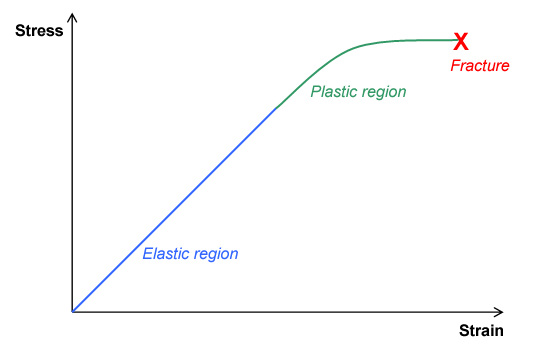
Three mechanical states of material

The Von Mises stress considers that yielding of a ductile material begins when the second invariant of deviatoric stress \(J_2\) reaches a critical value. The von Mises stress is used to predict yielding.

When the value Von Mises tensor is great than a pression give by the material, the material exits of elastic state and pass to plastic state.

The Von Mises stress is writed :

\[\begin{eqnarray*} \bar{\bar{\sigma}}_{Von \, Mises} &=& \sqrt{3 \, J_2} \\ &=& \sqrt{\frac{1}{2} \left( \left( \bar{\bar{\sigma}}_1 - \bar{\bar{\sigma}}_2 \right)^2 + \left( \bar{\bar{\sigma}}_1 - \bar{\bar{\sigma}}_3 \right)^2 + \left( \bar{\bar{\sigma}}_2 - \bar{\bar{\sigma}}_3 \right)^2 \right)} \\ &=& \sqrt{ \frac{1}{2} \left( (\bar{\bar{\sigma}}_{xx}-\bar{\bar{\sigma}}_{yy})^2 + (\bar{\bar{\sigma}}_{yy}-\bar{\bar{\sigma}}_{zz})^2 + (\bar{\bar{\sigma}}_{zz}-\bar{\bar{\sigma}}_{xx})^2 \right) + 3 \, \bar{\bar{\sigma}}_{xy}^2 + 3 \, \bar{\bar{\sigma}}_{yz}^2 + 3 \, \bar{\bar{\sigma}}_{zx}^2 } \\ &=& \sqrt{ \frac{1}{2} \left( (\bar{\bar{\sigma}}_{rr}-\bar{\bar{\sigma}}_{\theta \theta})^2 + (\bar{\bar{\sigma}}_{\theta \theta}-\bar{\bar{\sigma}}_{zz})^2 + (\bar{\bar{\sigma}}_{zz}-\bar{\bar{\sigma}}_{rr})^2 \right) + 3 \, \bar{\bar{\sigma}}_{r \theta}^2 + 3 \, \bar{\bar{\sigma}}_{\theta z}^2 + 3 \, \bar{\bar{\sigma}}_{zr}^2 } \end{eqnarray*}\]

In axisymmetrical approximation :

\[\scriptsize{ \bar{\bar{\sigma}}_{Von \, Mises} = \mu \, \sqrt{ 4 \left( \left(\frac{u_r}{r}\right)^2 + \left(\frac{\partial u_r}{\partial r}\right)^2 + \left(\frac{\partial u_z}{\partial z}\right)^2 - \frac{u_r}{r} \, \frac{\partial u_r}{\partial r} - \frac{u_r}{r} \, \frac{\partial u_z}{\partial z} - \frac{\partial u_r}{\partial r} \, \frac{\partial u_z}{\partial z} \right) + \frac{1}{2} \left( \frac{\partial u_r}{\partial z} + \frac{\partial u_z}{\partial r} \right) + \frac{\partial u_r}{\partial z} \, \frac{\partial u_z}{\partial r} } }\]

3.5. Tresca Tensor

Like Von Mises tensor, the Tresca Tensor serves to predict the yielding of material.

When the value Von Mises tensor is great than a pression give by the material, the material exits of elastic state and pass to plastic state.

The Tresca Tensor is defined like :

\[\begin{eqnarray*} \bar{\bar{\sigma}}_{tr} &=& \underset{1 \leq i < j \leq 3}{max}{ | \bar{\bar{\sigma}}_i - \bar{\bar{\sigma}}_j | } \\ &=& max \left( |\bar{\bar{\sigma}}_1-\bar{\bar{\sigma}}_2|, \, |\bar{\bar{\sigma}}_1-\bar{\bar{\sigma}}_3|, \, |\bar{\bar{\sigma}}_2-\bar{\bar{\sigma}}_3| \right) \end{eqnarray*}\]

4. Documentation

Elasticity adn toolbox Coefficient Form PDEs, Céline Van Landeghem, 2021, unpublished, Download the PDF

Coupled modelling and simulation of electromagnets in stationnary and instationnary modes (axisymmetric and 3D), J. Nadarasa, June 2 2015, unpublished, page 20-24, Download the PDF

Theorical Physics Reference, Ondřej Čertík, November 29 2011, page 85-90 Download the PDF

Cauchy stress tensor, Wikipedia, March 11 2021, Link to website

von Mises yield criterion, Wikipedia, March 11 2021, von Mises yield criterion