Test Case of Thermal Dilatation Static in Three Dimensions on Beam Geometry

1. Introduction

This page presents the test case of Thermal Dilatation implement with CFPDEs with constant temperature without volumic force in static and in three dimensions, solve components by components. This simulation have goal to verify the implementation of thermal dilatation.

2. Run the calculation

The command line to run this case is :

    mpirun -np 16 feelpp_toolbox_coefficientformpdes --config-file=thermal-dilatation.cfg --cfpdes.gmsh.hsize=5e-3

3. Data Files

The case data files are available in Github here :

CFG file - Edit the file
JSON file - Edit the file
GEO file - Edit the file

4. Equation

The domain of resolution is \(\Omega_c^{axis}\) with bounds \(\Gamma_c^{axis}\), \(\Gamma_{D \hspace{0.05cm} elas}^{axis}\) the bound of elastic Dirichlet conditions, \(\Gamma_{N \hspace{0.05cm} elas}^{axis}\) the bound of elastic Neumann conditions such that \(\Gamma_c^{axis} = \Gamma_{D \hspace{0.05cm} elas}^{axis} \cup \Gamma_{N \hspace{0.05cm} elas}^{axis}\).

Differential Formulation of Elasticity Equation in Stationary Case

\[\text{(Static Elasticity)} \left\{ \begin{matrix} - \nabla \cdot \bar{\bar{\sigma}} = \mathbf{F} & \text{on } \Omega_c & \text{(Static Elas-1)} \\ \mathbf{u} = \mathbf{u_0} & \text{on } \Gamma_{D \hspace{0.05cm} elas} & \text{(D elas)} \\ \bar{\bar{\sigma}} \cdot \mathbf{n} = g_N & \text{on } \Gamma_{N \hspace{0.05cm} elas} & \text{(N elas)} \\ \bar{\bar{\sigma}} \cdot \mathbf{n} + k \, \mathbf{u} = g_R & \text{on } \Gamma_{R \hspace{0.05cm} elas} & \text{(R elas)} \end{matrix} \right.\]

With :

Displacement \(\mathbf{u} = \begin{pmatrix} u_x \\ u_y \\ u_z \end{pmatrix}\)
Stress Tensor : \(\bar{\bar{\sigma}}\)
Stiffness tensor : \(k\)
Volumic Forces : \(\mathbf{F}\)

And notations :

Divergence of tensor : \(\nabla \cdot \bar{\bar{\sigma}} = \begin{pmatrix} \nabla \cdot \bar{\bar{\sigma}}_{x,:} \\ \nabla \cdot \bar{\bar{\sigma}}_{y,:} \\ \nabla \cdot \bar{\bar{\sigma}}_{z,:} \end{pmatrix} = \begin{pmatrix} \frac{\partial \bar{\bar{\sigma}}_{xx}}{\partial x} + \frac{\partial \bar{\bar{\sigma}}_{xy}}{\partial y} + \frac{\partial \bar{\bar{\sigma}}_{xz}}{\partial z} \\ \frac{\partial \bar{\bar{\sigma}}_{yx}}{\partial x} + \frac{\partial \bar{\bar{\sigma}}_{yy}}{\partial y} + \frac{\partial \bar{\bar{\sigma}}_{yz}}{\partial z} \\ \frac{\partial \bar{\bar{\sigma}}_{zx}}{\partial x} + \frac{\partial \bar{\bar{\sigma}}_{zy}}{\partial y} + \frac{\partial \bar{\bar{\sigma}}_{zz}}{\partial z} \end{pmatrix}\)
Scalar produce of tensor : \(\bar{\bar{\sigma}} \cdot \mathbf{n} = \begin{pmatrix} \bar{\bar{\sigma}}_{x,:} \cdot \mathbf{n} \\ \bar{\bar{\sigma}}_{y,:} \cdot \mathbf{n} \\ \bar{\bar{\sigma}}_{z,:} \cdot \mathbf{n} \end{pmatrix} = \begin{pmatrix} \bar{\bar{\sigma}}_{xx} \, n_x + \bar{\bar{\sigma}}_{xy} \, n_y + \bar{\bar{\sigma}}_{xz} \, n_z \\ \bar{\bar{\sigma}}_{yx} \, n_x + \bar{\bar{\sigma}}_{yy} \, n_y + \bar{\bar{\sigma}}_{yz} \, n_z \\ \bar{\bar{\sigma}}_{zx} \, n_x + \bar{\bar{\sigma}}_{zy} \, n_y + \bar{\bar{\sigma}}_{zz} \, n_z \end{pmatrix}\)

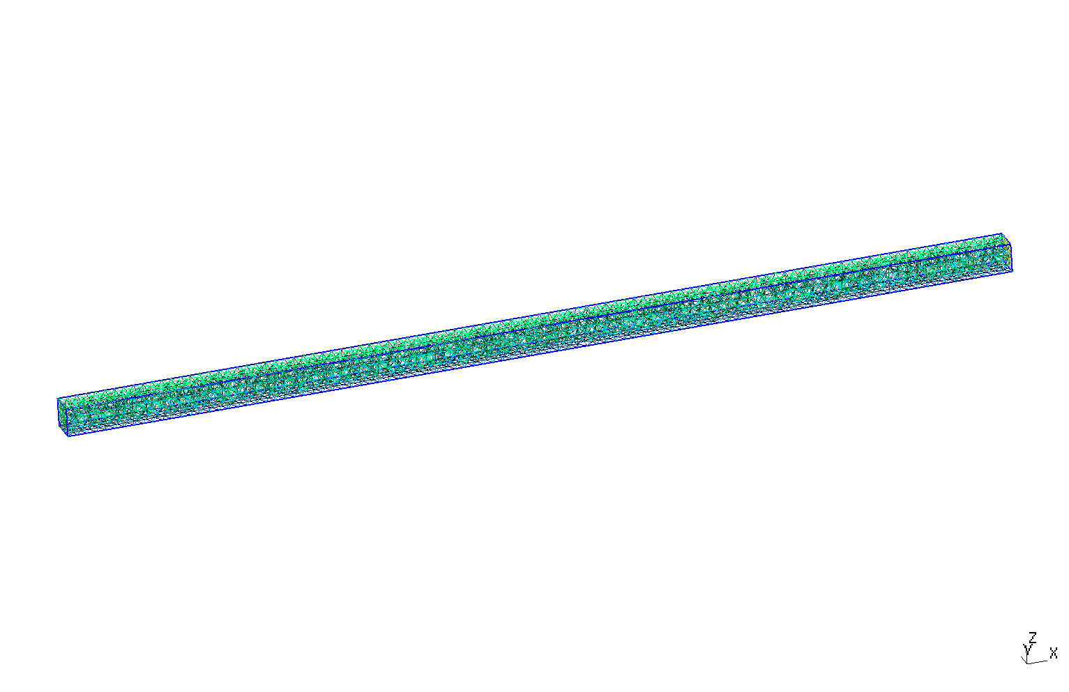
5. Geometry

The geometry is a torus of the conductor in cartesian coordinates \((x,y,z)\) or rectangle in axisymmetric coordinates \((r,z)\), surrounded by air.

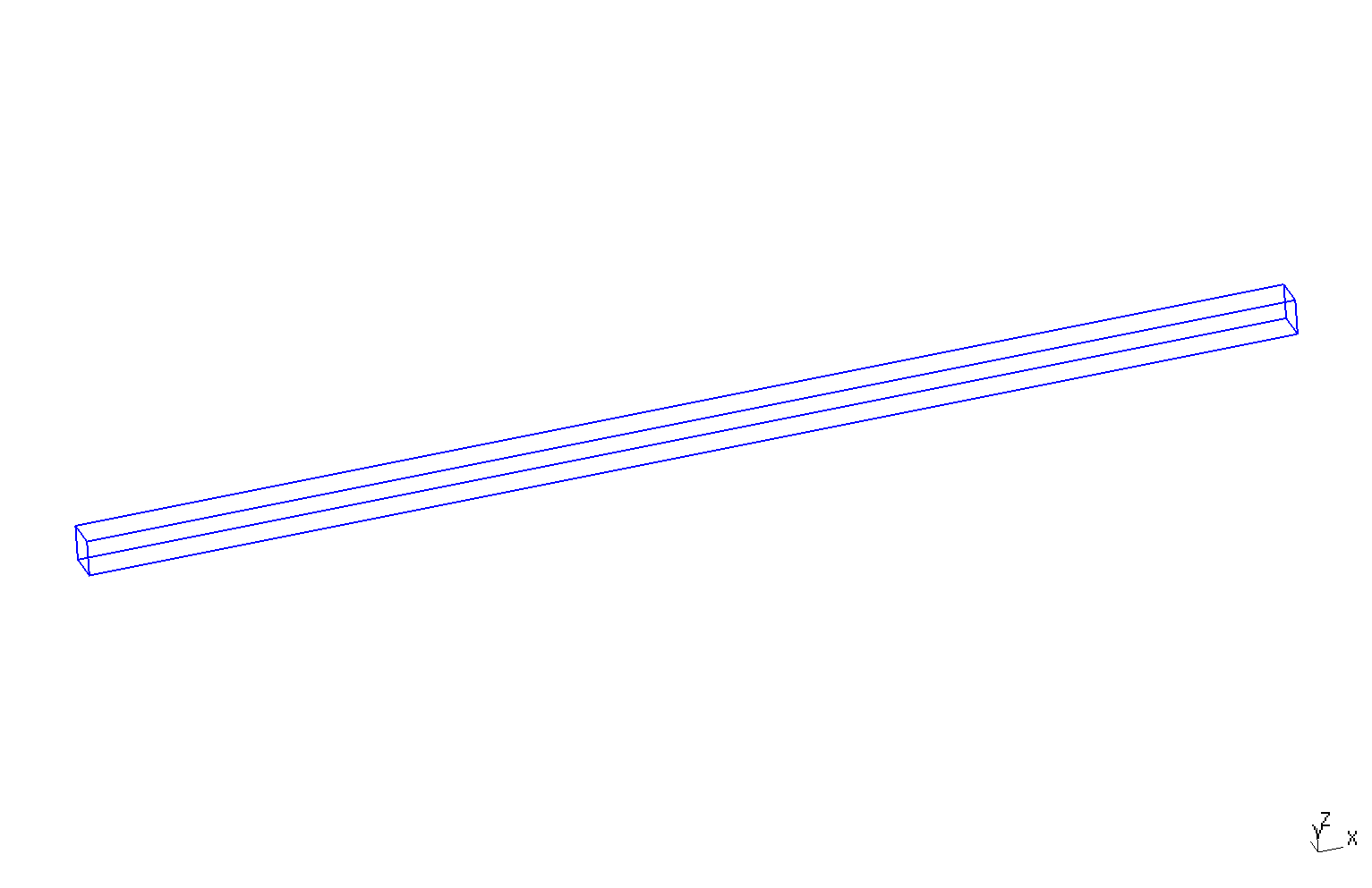
Geometry

The geometrical domains are :

Omega : the torus is composed by conductor material
- Left : left side of beam
- Right : right side of beam
- Upper : upper side of beam
- Bottom : bottom side of beam
- Front : front side of beam
- Backward : backward side of beam

Symbol

Description

value

unit

\(L\)

interior radius of torus

\(10\)

\(w\)

exterior radius of torus

\(0.3\)

6. Boundary Conditions

We impose the boundary conditions :

Strong Dirichlet : \(\mathbf{u} = 0\) on Left. The Dirichlet condition represents the embedding of mechanical part.
Neumann : \(\bar{\bar{\sigma}} \cdot \mathbf{n} = 0\) on the rest of bound. The Neumann condition represents the freedom of displacement.

On JSON file, the boundary conditions are writed :

Boundary conditions on JSON file

    "BoundaryConditions":
    {
        "elastic":
        {
            "Dirichlet":
            {
                "Left":
                {
                    "expr":"{0,0,0}"
                }
            }
        }
    }

7. Weak Formulation

We obtain :

Weak Formulation of Elasticity Equation in Stationnary Case

\[\text{(Weak Static Elasticity)} \\ \left\{ \begin{matrix} \int_{\Omega_c}{ \bar{\bar{\sigma}}_{xx} \, \frac{\partial \xi_x}{\partial x} + \bar{\bar{\sigma}}_{xy} \, \frac{\partial \xi_x}{\partial y} + \bar{\bar{\sigma}}_{xz} \, \frac{\partial \xi_x}{\partial z} + \bar{\bar{\sigma}}_{yx} \, \frac{\partial \xi_y}{\partial x} + \bar{\bar{\sigma}}_{yy} \, \frac{\partial \xi_y}{\partial y} + \bar{\bar{\sigma}}_{yz} \, \frac{\partial \xi_y}{\partial z} + \bar{\bar{\sigma}}_{zx} \, \frac{\partial \xi_z}{\partial x} + \bar{\bar{\sigma}}_{zy} \, \frac{\partial \xi_z}{\partial y} + \bar{\bar{\sigma}}_{zz} \, \frac{\partial \xi_z}{\partial z} } = \int_{\Omega_c}{ F \cdot \mathbf{ξ} } + \int_{\Gamma_{N \hspace{0.05cm} elas}}{ g_N \cdot \mathbf{ξ} } + \int_{\Gamma_{R \hspace{0.05cm} elas}}{ \left( g_R - \left( k \, u \right) \right) \cdot \mathbf{ξ} } \\ \text{for } \mathbf{ξ} = \begin{pmatrix} \xi_x \\ \xi_y \\ \xi_z \end{pmatrix} \in H^1_{u_0}(\Omega_c) \end{matrix} \right.\]

8. Parameters

The parameters of problem are :

Symbol

Description

Value

Unit

\(E\)

Young Modulus

\(2.1e6\)

\(Pa\)

\(v\)

Poisson’s coefficient

\(0.33\)

\(dimensionless\)

\(\lambda\)

Lame’s coefficient

\(\frac{E \, v}{(1-2v)(1+v)}\)

\(Pa\)

\(\mu\)

Lame’s coefficient

\(\frac{E}{2 (1+v)}\)

\(Pa\)

\(T\)

heating temperature

\(293\)

\(K\)

\(T_0\)

rest temperature

\(303\)

\(K\)

On JSON file, the parmeters are writed :

Parameters on JSON file

    "Parameters": {
        "L":10,
        "E": 2.1e6,
        "nu": 0.33,
        "mu": "E/(2*(1+nu)):E:nu",
        "lambda":"E*nu/((1+nu)*(1-2*nu)):E:nu",
        "T0":293,
        "T":303,
        "alpha_T":"17e-6",
        "sigma_T":"-E/(1-2*nu)*alpha_T*(T-T0):E:nu:alpha_T:T:T0"
    }

9. Coefficient Form PDEs

We use the application Coefficient Form PDEs. The coefficient associate to Weak Formulation are :

Coefficient

Description

Expression

\(c\)

\(\mu\)

\(\mathbf{γ}\)

conservative flux source term

\(\begin{pmatrix} -\lambda \left( \frac{\partial u_x}{\partial x} + \frac{\partial u_y}{\partial y} + \frac{\partial_z}{\partial z} \right) - \sigma_T - \mu \frac{\partial u_x}{\partial x} & -\mu \left( \frac{\partial u_x}{\partial y} + \frac{\partial u_y}{\partial x} \right) & -\mu \left( \frac{\partial u_x}{\partial z} + \frac{\partial u_z}{\partial x} \right) \\ -\mu \left( \frac{\partial u_x}{\partial y} + \frac{\partial u_y}{\partial x} \right) & -\lambda \left( \frac{\partial u_x}{\partial x} + \frac{\partial u_y}{\partial y} + \frac{\partial_z}{\partial z} \right) - \sigma_T - \mu \frac{\partial u_y}{\partial y} & -\mu \left( \frac{\partial u_y}{\partial z} + \frac{\partial u_z}{\partial y} \right) \\ -\mu \left( \frac{\partial u_x}{\partial z} + \frac{\partial u_z}{\partial x} \right) & -\mu \left( \frac{\partial u_y}{\partial z} + \frac{\partial u_z}{\partial y} \right) & -\lambda \left( \frac{\partial u_x}{\partial x} + \frac{\partial u_y}{\partial y} + \frac{\partial_z}{\partial z} \right) - \sigma_T - \mu \frac{\partial u_z}{\partial z} \end{pmatrix}\)

On JSON file, the coefficients are writed :

CFPDEs coefficients on JSON file

    "Materials":
    {
        "Omega":
        {
            "elastic_c": "mu:mu",
            "elastic_gamma":"{-lambda*(elastic_grad_u_00+elastic_grad_u_11+elastic_grad_u_22) - sigma_T - mu*elastic_grad_u_00,-mu*elastic_grad_u_10,-mu*elastic_grad_u_20, -mu*elastic_grad_u_01,-lambda*(elastic_grad_u_00+elastic_grad_u_11+elastic_grad_u_22) - sigma_T - mu*elastic_grad_u_11,-mu*elastic_grad_u_21, -mu*elastic_grad_u_02,-mu*elastic_grad_u_12,-lambda*(elastic_grad_u_00+elastic_grad_u_11+elastic_grad_u_22) - sigma_T - mu*elastic_grad_u_22}:lambda:mu:elastic_grad_u_00:elastic_grad_u_01:elastic_grad_u_10:elastic_grad_u_11:elastic_grad_u_20:elastic_grad_u_21:elastic_grad_u_22:elastic_grad_u_02:elastic_grad_u_12:sigma_T",

            "sigma_xx":"(lambda+2*mu)*elastic_grad_u_00+mu*elastic_grad_u_11+mu*elastic_grad_u_22+sigma_T:lambda:mu:elastic_grad_u_00:elastic_grad_u_11:elastic_grad_u_22:sigma_T",
            "sigma_yy":"mu*elastic_grad_u_00+(lambda+2*mu)*elastic_grad_u_11+mu*elastic_grad_u_22+sigma_T:lambda:mu:elastic_grad_u_00:elastic_grad_u_11:elastic_grad_u_22:sigma_T",
            "sigma_zz":"mu*elastic_grad_u_00+mu*elastic_grad_u_11+(lambda+2*mu)*elastic_grad_u_22+sigma_T:lambda:mu:elastic_grad_u_00:elastic_grad_u_11:elastic_grad_u_22:sigma_T",
            "sigma_xy":"mu*(elastic_grad_u_01+elastic_grad_u_10):mu:elastic_grad_u_01:elastic_grad_u_10",
            "sigma_xz":"mu*(elastic_grad_u_02+elastic_grad_u_20):mu:elastic_grad_u_02:elastic_grad_u_20",
            "sigma_yz":"mu*(elastic_grad_u_12+elastic_grad_u_21):mu:elastic_grad_u_12:elastic_grad_u_21"
        }
    }

10. Numeric Parameters

Mesh size \(0.02 \, m\)

Mesh of Geometry

11. Results

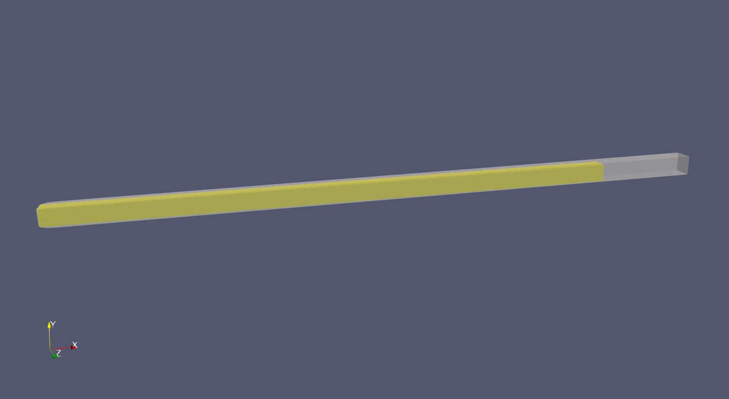
Deformation result of dilatation compute with cfpdes (with scale=1000). The yellow solid is the initial shape and the white solid is the final shape.

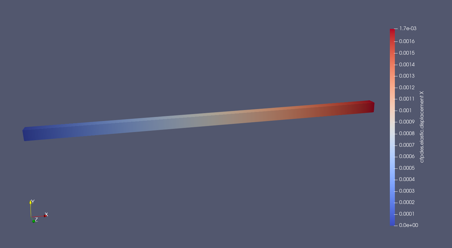
Value of \(u_x\) (\(m\)) on beam

I plot my result and analytical solve (\(u_x = \alpha_T (T-T_0) x\)) on \(O_x\) axis.

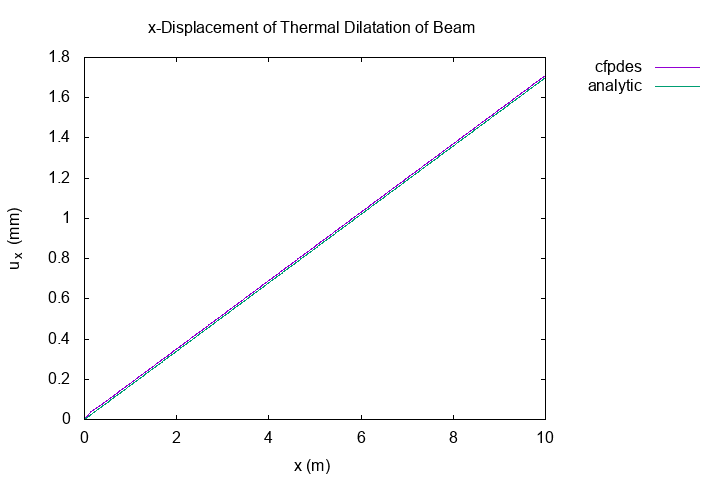
\(u_x\) \((mm)\) on \(O_x\) axiss

The two curves overlap.

We have trust of the method for simulation of thermal dilatation on beam.