Test case : Two Tores :: Project M2 Lncmi

1. Introduction

In this page, I present the test case of Maxwell Quasi Static Problem in A-V Formulation with gauge condition for a geometry of two torus surrounded by air for instationnary case in Axisymmetrical case.

2. Run the calculation

The command line to run this case is :

    mpirun -np 16 feelpp_toolbox_coefficientformpdes --config-file=mqs.cfg --cfpdes.gmsh.hsize=1e-3

3. Data Files

The case data files are available in Github here :

CFG file - Edit the file
JSON file - Edit the file
GEO file - Edit the file

4. Equation

We solve the A-V Formulation in axisymmetric and we assume that \(V\) is known.

Differential Formulation

\[\text{(AV Axis)} \left\{ \begin{matrix} \sigma \frac{\partial \Phi}{\partial t} - \frac{1}{\mu} \Delta \Phi + \frac{2}{\mu \, r} \frac{\partial \Phi}{\partial r} + \sigma \frac{\partial V}{\partial \theta} = 0 & \text{ on } \Omega^{axis} & \text{(AV-1 Axis)} \\ V = \frac{U}{2\pi} \, \theta & \text{ on } \Omega_c^{axis} \\ A_{\theta} = 0 & \text{ on } \Gamma_D^{axis} & \text{(D Axis)} \\ \frac{\partial A_{\theta}}{\partial \mathbf{n}^{axis}} = 0 & \text{ on } \Gamma_N^{axis} & \text{(N Axis)} \end{matrix} \right.\]

With :

\(\Phi = r A_{\theta}\) : \(A_{\theta}\) component \(\theta\) of potential magnetic field
\(\sigma\) : electric conductivity \(S/m\)
\(\mu\) : electric permeability \(kg/A^2/S^2\)
\(U\) : tension \(Volt\)

5. Geometry

The geometry is two tores of conductor in cartesian coordinates \((x,y,z)\) or two rectangles in axisymmetric coordinates \((r,z)\), surrounded by air.

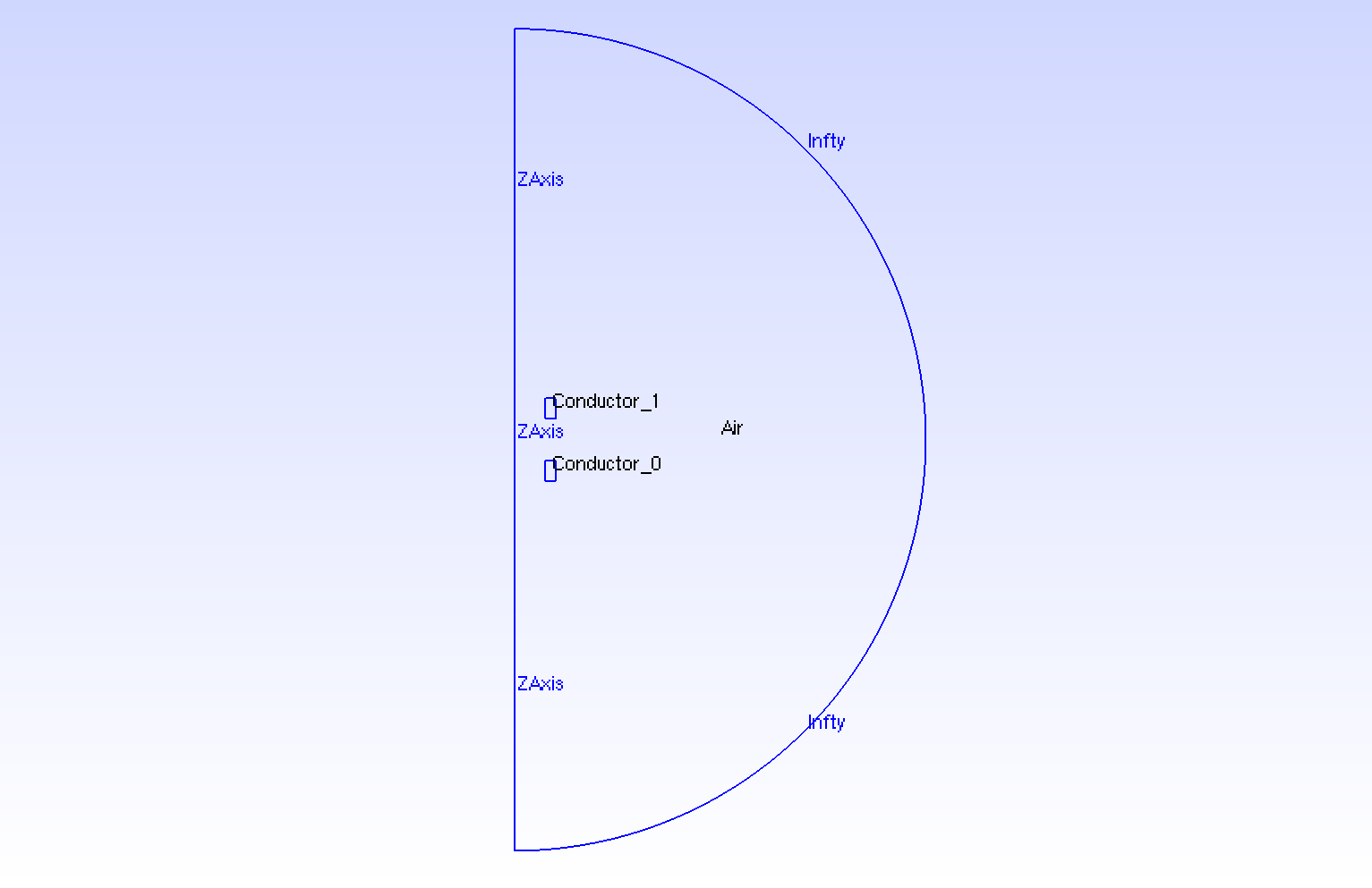
Geometry in Axisymmetrical cut

Geometry in Axisymmetrical cut loop on Conductors

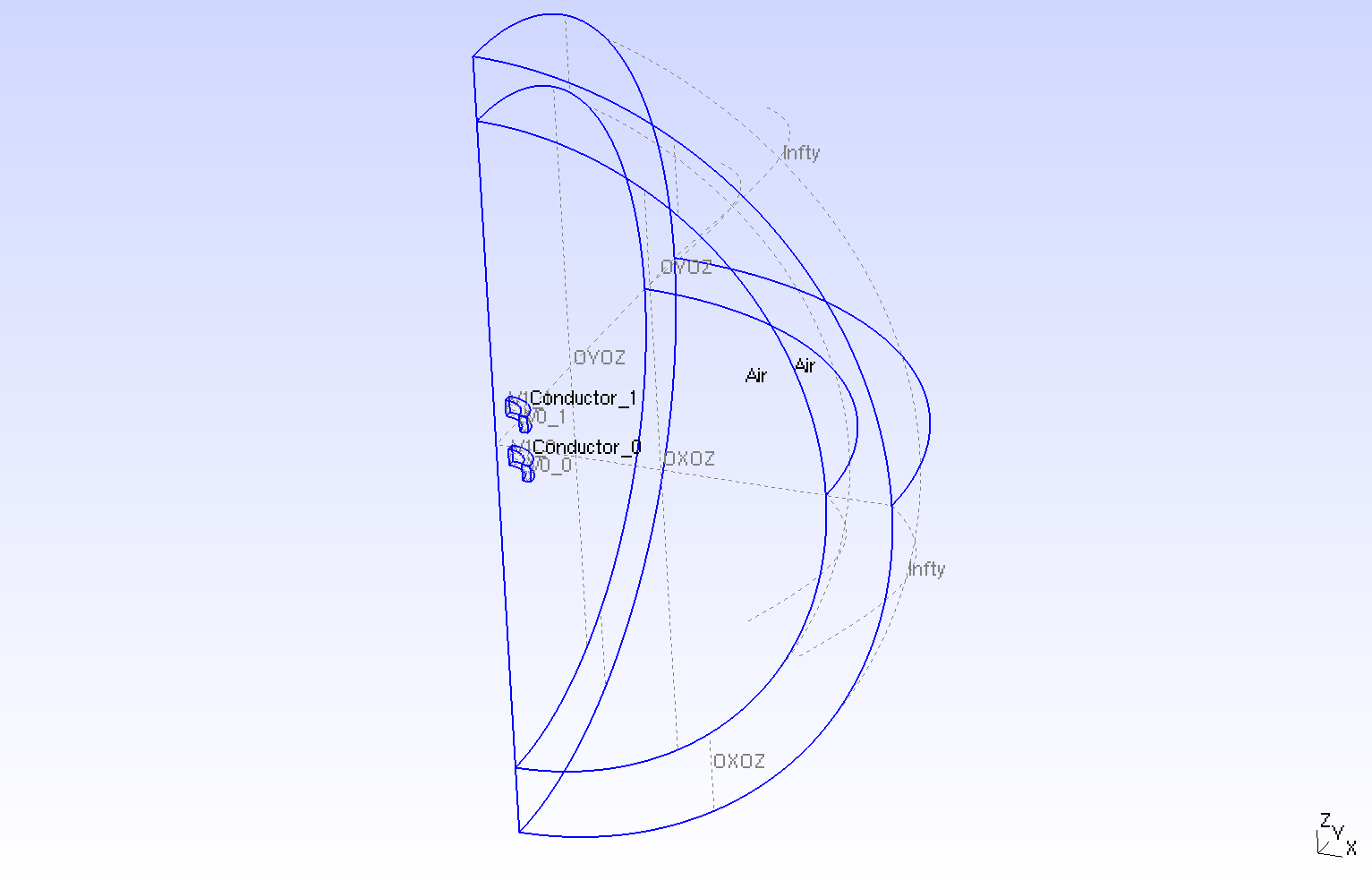
Geometry in three dimensions

Geometry in three dimensions loop on Conductors

The geometrical domains are :

Conductor_0 : the torus is composed by conductor material
Conductor_1 : the torus is composed by conductor material

Conductor_0 \(\cup\) Conductor_1 \( = \Omega_c^{axis}\)

Air : the air surround Conductor_0 and Conductor_1
- zAxis : a bound of Air, correspond to \(Oz\) axis (\(\{(z,r), \, z=0 \}\))
- infty : the rest of bound of Air

Air \(= \Omega^{axis} / \Omega_c^{axis}\).

Symbol

Description

value

unit

\(r_{int}\)

interior radius of tores

\(75e-3\)

m

\(r_{ext}\)

exterior radius of tores

\(100.2e-3\)

m

\(z_1\)

half-height of tores

\(25e-3\)

m

\(r_{infty}\)

radius of infty border

\(5*r_{ext}\)

6. Initial/Boundary Conditions

We impose the Dirichlet boundary conditions :

On zAxis : \(\Phi = 0\) (\(A_{\theta} = 0\) by symetric argument)
On infty : \(\Phi = 0\) (\(A_{\theta} = 0\) we consider the bound of resolution like infty for magnetic field)

We initialize :

On Conductor_0 and Conductor_1 : \(\Phi(t=0,r,z) = 0\) (\(A_{\theta}(t=0,r,z) = 0\))
On Air : \(\Phi(t=0,r,z) = 0\) (\(A_{\theta}(t=0,r,z) = 0\))

On JSON file, the boundary conditions are writed :

Boundary conditions on JSON file

    "BoundaryConditions":
    {
        "magnetic":
        {
            "Dirichlet":
            {
                "ZAxis":
                {
                    "expr":"0"
                },
                "Infty":
                {
                    "expr":"0"
                }
            }
        }
    }

For initial condition, we write nothing in JSON, by default the application put zeros on initialization.

7. Weak Formulation

We obtain :

Weak Formulation

\[\scriptsize{ \int_{\Omega^{axis}}{ \sigma \frac{\partial \Phi}{\partial t} \phi \ r\ drdz} + \int_{\Omega^{axis}}{ \frac{1}{\mu} \tilde{\nabla} \Phi \cdot \tilde{\nabla} \phi \ r \ drdz } + \int_{\Omega^{axis}}{\frac{2}{\mu \, r} \frac{\partial \Phi}{\partial r} \, \phi \ r \ drdz} = - \int_{\Omega_c^{axis}}{ \sigma \frac{\partial V}{\partial \theta} \phi \ r \ drdz } }\]

With \(\tilde{\nabla} = \begin{pmatrix} \frac{\partial}{\partial r} \\ \frac{\partial}{\partial z} \end{pmatrix}\)

8. Parameters

The parameters of problem are :

On Conductor_0 and Conductor_1 :

Symbol

Description

Value

Unit

\(V_0\)

scalar electrical potential of Conductor_0

\( U_0 \, \frac{\theta}{2\pi}\)

\(Volt\)

\(U_0\)

electrical potential of Conductor_0

\(\left\{ \begin{matrix} t/0.1 \text{ on } 0s \leq t \leq 0.1s \\ 1 \text{ on } 0.1s \leq t \leq 0.5s \\ 0 \text{ on } 0.5s \leq t \leq 1s \end{matrix} \right.\)

\(Volt / rad\)

\(V_1\)

scalar electrical potential of Conductor_1

\( U_1 \, \frac{\theta}{2\pi}\)

\(Volt\)

\(U_1\)

electrical potential of Conductor_1

\(\left\{ \begin{matrix} t/0.1 \text{ on } 0s \leq t \leq 0.1s \\ 1 \text{ on } 0.1s \leq t \leq 0.7s \\ 0 \text{ on } 0.7s \leq t \leq 1s \end{matrix} \right.\)

\(Volt / rad\)

\(\sigma\)

electrical conductivity

\(58e6\)

\(S/m\)

\(\mu=\mu_0\)

magnetic permeability of vacuum

\(4\pi.10^{-7}\)

\(kg \, m / A^2 / S^2\)

On Air :

Symbol

Description

Value

Unit

\(\mu=\mu_0\)

magnetic permeability of vacuum

\(4\pi.10^{-7}\)

\(kg \, m / A^2 / S^2\)

9. Coefficient Form PDEs

We use the application Coefficient Form PDEs. The coefficient associate to Weak Formulation are :

On Conductor_0 and Conductor_1 :

Coefficient

Description

Expression

\(d\)

damping or mass coefficient

\(\sigma\)

\(c\)

diffusion coefficient

\(\frac{r}{\mu}\)

\(\beta\)

convection coefficient

\(\begin{pmatrix} \frac{2}{\mu} \\ 0 \end{pmatrix}\)

\(f\)

source term

\(- \sigma \frac{U_i}{2\pi} \, r\) with \(i=0,1\)

On Air :

Coefficient

Description

Expression

\(c\)

diffusion coefficient

\(\frac{r}{\mu}\)

\(\beta\)

convection coefficient

\(\begin{pmatrix} \frac{2}{\mu} \\ 0 \end{pmatrix}\)

On JSON file, the coefficients are writed :

CFPDEs coefficients on JSON file

    "Materials":
    {
        "Conductor_0":
        {
            "U":"t/(0.1)*(t<(0.1))+(t<(0.5))*(t>(0.1)):t", // Volt
            "sigma":58e+6,      // S.m-1
            "mu":"4*pi*1e-7",   // kg.m/A2/S2
	        "magnetic_c":"x/mu:x:mu",
            "magnetic_beta":"{2/mu,0}:mu",
            "magnetic_f":"-sigma*U/2/pi*x:sigma:U:x:mu",
            "magnetic_d":"sigma*x:x:sigma"
        },
        "Conductor_1":
        {
            "U":"t/(0.1)*(t<(0.1))+(t<(0.7))*(t>(0.1)):t", // Volt
            "sigma":58e+6,      // S.m-1
            "mu":"4*pi*1e-7",   // kg.m/A2/S2
	        "magnetic_c":"x/mu:x:mu",
            "magnetic_beta":"{2/mu,0}:mu",
            "magnetic_f":"-sigma*U/2/pi*x:sigma:U:x:mu",
            "magnetic_d":"sigma*x:x:sigma"
        },
        "Air":
        {
            "mu":"4*pi*1e-7",   // kg.m/A2/s2
            "magnetic_c":"x/mu:x:mu",
            "magnetic_beta":"{2/mu,0}:mu"
        }
    }

10. Numeric Parameters

Time
- Initial Time : \(0s\)
- Final Time : \(1s\)
- Time Step : \(0.005s\)
Mesh size :
- Interior of torus : \(0.001 m\)
- Far of torus : \(0.004 m\)

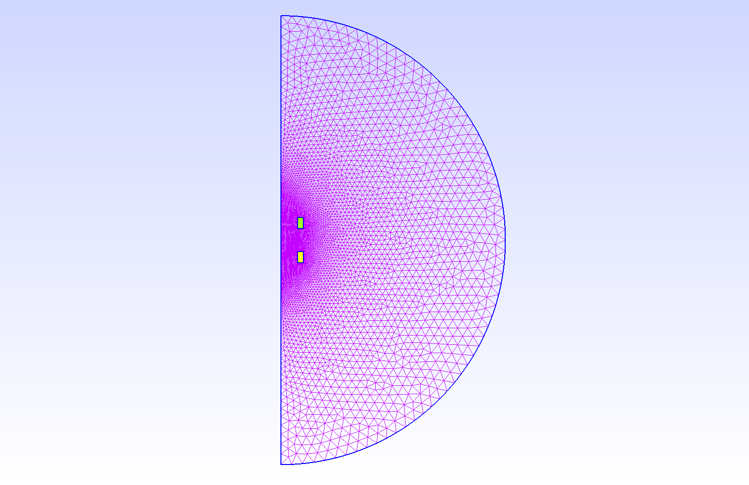
Mesh of Geometry

11. Run the calculation

11.1. CFPDEs

12. Exact Solutions

12.1. Intensity

In this subsection, we see the analytical compute of intensities.

We have :

\[\text{(I 2torus)} \left\{ \begin{eqnarray*} R \, I_0 + L \, \frac{d I_0}{d t} + M \, \frac{d I_1}{d t} &=& U_0 \\ R \, I_1 + L \, \frac{d I_1}{d t} + M \, \frac{d I_0}{d t} &=& U_1 \\ \end{eqnarray*} \right.\]

With \(I_0\) the intensity of Conductor_0 and \(I_1\) the intensity of Conductor_1. \(R\) is the resistance of two tores, \(L\) the inductance of two tores and \(M\) the mutual inductance between the two tores.

And :

\[ U_0 = \left\{ \begin{matrix} \frac{t}{0.1} & \text{ for } 0s \leq t \leq 0.1s \\ 1 & \text{ for } 0.1s \leq t \leq 0.5s \\ 0 & \text{ for } 0.5 \leq t \end{matrix} \right. \hspace{0.5cm} \text{,} \hspace{0.5cm} U_1 = \left\{ \begin{matrix} \frac{t}{0.1} & \text{ for } 0s \leq t \leq 0.1s \\ 1 & \text{ for } 0.1s \leq t \leq 0.7s \\ 0 & \text{ for } 0.5 \leq t \end{matrix} \right.\]

To solve this system of equation, we pass in vectorial formulation, we pose \(\mathbf{I} = \begin{pmatrix} I_0 \\ I_1 \end{pmatrix}\), \(\mathbf{U} = \begin{pmatrix} U_0 \\ U_1 \end{pmatrix}\), \(\mathbf{R} = \begin{pmatrix} R & 0 \\ 0 & R \end{pmatrix}\) and \(\mathbf{L} = \begin{pmatrix} L & M \\ M & L \end{pmatrix}\). The (I 2torus) equation becomes :

\[ \mathbf{R} \, \mathbf{I} + \mathbf{L} \, \frac{d \mathbf{I}}{d t} = \mathbf{U}\]

\(\mathbf{R}\) and \(\mathbf{L}\) are supposed invertible.

Resolution of First Part \((0s\leq t \leq 0.1s)\) :

\[ \mathbf{R} \, \mathbf{I} + \mathbf{L} \, \frac{d \mathbf{I}}{d t} = \begin{pmatrix} t/0.1 \\ t/0.1 \end{pmatrix}\]

The harmonic equation \(\mathbf{R} \, \mathbf{\tilde{I}} + \mathbf{L} \, \frac{d \mathbf{\tilde{I}}}{d t} = 0\) have a solution \(\mathbf{\tilde{I}} = e^{-\mathbf{R}\mathbf{L}^{-1} \, t}\)

We pose \(\mathbf{I} = e^{- \mathbf{R} \mathbf{L}^{-1} \, t} \, \mathbf{C}\), with \(\mathbf{C}(t) \in \mathbb{R}^2\) such as \(\mathbf{I}\) verify (I 2torus) (we consider that \(\mathbf{I}(0)=0\) thus \(\mathbf{C}(0)=0\) ) :

\[\begin{eqnarray*} \begin{pmatrix} t/0.1 \\ t/0.1 \end{pmatrix} &=& \mathbf{R} \, e^{- \mathbf{R} \mathbf{L}^{-1} \, t} \, \mathbf{C} + \mathbf{L} \, e^{- \mathbf{R} \mathbf{L}^{-1} \, t} \, \frac{d \mathbf{C}}{d t} - \mathbf{L} \, \left( \mathbf{R} \mathbf{L}^{-1} \right) e^{- \mathbf{R} \mathbf{L}^{-1} \, t} \, \mathbf{C} \\ \begin{pmatrix} t/0.1 \\ t/0.1 \end{pmatrix} &=& \mathbf{L} \, e^{- \mathbf{R} \mathbf{L}^{-1} \, t} \, \frac{d \mathbf{C}}{d t} \\ \frac{d \mathbf{C}}{d t} &=& e^{\mathbf{R} \mathbf{L}^{-1} \, t} \, \mathbf{L}^{-1} \, \begin{pmatrix} t/0.1 \\ t/0.1 \end{pmatrix} \end{eqnarray*}\]

Thus :

\[\begin{eqnarray*} \mathbf{C}(t) &=& \int_{\tau=0}^t{\tau \, e^{\mathbf{R} \mathbf{L}^{-1} \tau} \, d\tau} \ \mathbf{L}^{-1} \, \begin{pmatrix} 1/0.1 \\ 1/0.1 \end{pmatrix} \\ &=& \left( \left[ \tau \, \left( \mathbf{R} \mathbf{L}^{-1} \right)^{-1} \, e^{\mathbf{R} \mathbf{L}^{-1} \tau} \right]_{\tau=0}^t - \int_{\tau=0}^t{ \left( \mathbf{R} \mathbf{L}^{-1} \right)^{-1} \,e^{\mathbf{R} \mathbf{L}^{-1} \tau} \, d\tau} \right) \ \mathbf{L}^{-1} \, \begin{pmatrix} 1/0.1 \\ 1/0.1 \end{pmatrix} \\ &=& \left( t \, \left( \mathbf{R} \mathbf{L}^{-1} \right)^{-1} \, e^{\mathbf{R} \mathbf{L}^{-1} t} - \left[ \left( \mathbf{R} \mathbf{L}^{-1} \right)^{-2} \, e^{\mathbf{R} \mathbf{L}^{-1} \tau} \right]_{\tau=0}^t \right) \ \mathbf{L}^{-1} \, \begin{pmatrix} 1/0.1 \\ 1/0.1 \end{pmatrix} \\ &=& \left( t \, \left( \mathbf{R} \mathbf{L}^{-1} \right)^{-1} \, e^{\mathbf{R} \mathbf{L}^{-1} t} - \left( \mathbf{R} \mathbf{L}^{-1} \right)^{-2} \left( e^{\mathbf{R} \mathbf{L}^{-1} t} - Id \right) \right) \ \mathbf{L}^{-1} \, \begin{pmatrix} 1/0.1 \\ 1/0.1 \end{pmatrix} \end{eqnarray*}\]

Recall : \(e^{\mathbf{A}}\) commutes with \(\mathbf{A}\), thus :

\[ I(t) = \left( t \, \left( \mathbf{R} \mathbf{L}^{-1} \right)^{-1} - \left( \mathbf{R} \mathbf{L}^{-1} \right)^{-2} \left( Id - e^{-\mathbf{R} \mathbf{L}^{-1} t} \right) \right) \ \mathbf{L}^{-1} \, \begin{pmatrix} 1/0.1 \\ 1/0.1 \end{pmatrix}\]

Resolution of three last part (\(0s\leq t \leq 0.1s\), \(0.1s\leq t \leq 0.5s\) and \(0.5s\leq t \leq 1s\)) :

We have :

\[ \mathbf{R} \, \mathbf{I} + \mathbf{L} \, \frac{d \mathbf{I}}{d t} = \mathbf{U}\]

With \(\mathbf{U}\) constant (\(U = \begin{pmatrix} 1 \\ 1 \end{pmatrix}\), \(\begin{pmatrix} 0 \\ 1 \end{pmatrix}\) and \(\begin{pmatrix} 0 \\ 0 \end{pmatrix}\))

The solution of this equation is :

\[ I(t) = e^{-\mathbf{R} \mathbf{L}^{-1} t} \, \mathbf{C} + \mathbf{R}^{-1} \mathbf{U}\]

Conclusion : the solution of the equation (I 2torus) is :

\[\small{ \mathbf{I}(t) = \left\{ \begin{matrix} \left( t \, \left( \mathbf{R} \mathbf{L}^{-1} \right)^{-1} - \left( \mathbf{R} \mathbf{L}^{-1} \right)^{-2} \left( Id - e^{-\mathbf{R} \mathbf{L}^{-1} t} \right) \right) \ \mathbf{L}^{-1} \, \begin{pmatrix} 1/0.1 \\ 1/0.1 \end{pmatrix} & 0s \leq t \leq 0.1s \\ e^{-\mathbf{R} \mathbf{L}^{-1} t} \, \mathbf{C}_1 + \mathbf{R}^{-1} \begin{pmatrix} 1 \\ 1 \end{pmatrix} & 0.1s \leq t \leq 0.5s \\ e^{-\mathbf{R} \mathbf{L}^{-1} t} \, \mathbf{C}_2 + \mathbf{R}^{-1} \begin{pmatrix} 0 \\ 1 \end{pmatrix} & 0.5s \leq t \leq 0.7s \\ e^{-\mathbf{R} \mathbf{L}^{-1} t} \, \mathbf{C}_3 & 0.7s \leq t \leq 1s \\ \end{matrix} \right. }\]

With \(\mathbf{C}_1\), \(\mathbf{C}_2\) and \(\mathbf{C}_3\) constants which assure the continuity of intensity.

13. Results

13.1. Magnetic Fields

I plot the horizontal magnetic field by time on point \((0,0,0)\).

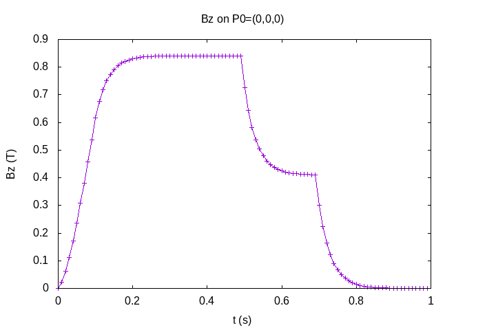
Horizontal Magnetic Field \(B_z (T)\) by time

We can see the four step :

the ramp for the two tensions
the tray for the two tensions
the tray for the tension \(U_1\) and the tray at 0 for the tension \(U_0\)
the tray for the tray at 0 for the tensions \(U_0\) and \(U_1\)

13.2. Intensities

The analytical solve of intensities is computed by python3’s script : Edit the file, with the formula :

\[\small{ \mathbf{I}(t) = \left\{ \begin{matrix} \left( t \, \left( \mathbf{R} \mathbf{L}^{-1} \right)^{-1} - \left( \mathbf{R} \mathbf{L}^{-1} \right)^{-2} \left( Id - e^{-\mathbf{R} \mathbf{L}^{-1} t} \right) \right) \ \mathbf{L}^{-1} \, \begin{pmatrix} 1/0.1 \\ 1/0.1 \end{pmatrix} & 0s \leq t \leq 0.1s \\ e^{-\mathbf{R} \mathbf{L}^{-1} t} \, \mathbf{C}_1 + \mathbf{R}^{-1} \begin{pmatrix} 1 \\ 1 \end{pmatrix} & 0.1s \leq t \leq 0.5s \\ e^{-\mathbf{R} \mathbf{L}^{-1} t} \, \mathbf{C}_2 + \mathbf{R}^{-1} \begin{pmatrix} 0 \\ 1 \end{pmatrix} & 0.5s \leq t \leq 0.7s \\ e^{-\mathbf{R} \mathbf{L}^{-1} t} \, \mathbf{C}_3 & 0.7s \leq t \leq 1s \\ \end{matrix} \right. }\]

And the values :

Symbol

Description

Value

Unit

\(R_0\)

resistance of Conductor_0

\(7.479339e-06\)

\(Ohm\)

\(R_1\)

resistance of Conductor_0

\(7.479339e-06\)

\(Ohm\)

\(L_0\)

auto-inductance of Conductor_0

\(1.920400e-07\)

\(Henry\)

\(L_0\)

auto-inductance of Conductor_0

\(1.920400e-07\)

\(Henry\)

\(M_{01}\)

inductance from Conductor_0 to Conductor_1

\(1.705000e-08\)

\(Henry\)

\(M_{10}\)

inductance from Conductor_1 to Conductor_0

\(1.705000e-08\)

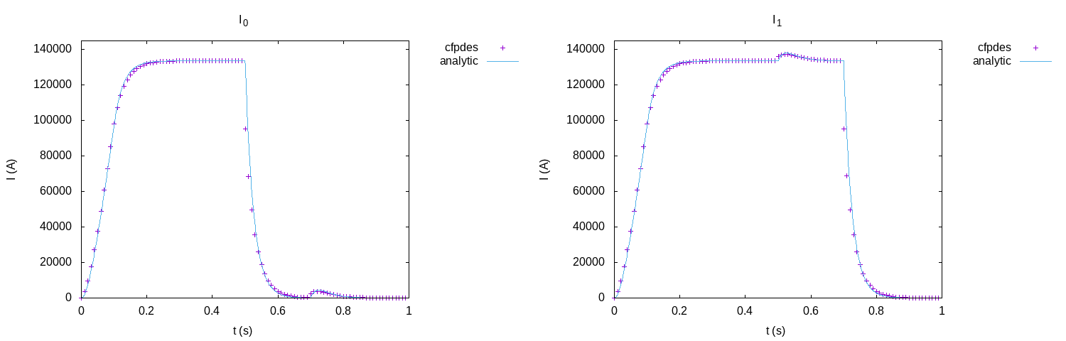
Intensities : Comparison between numerical and analytical results

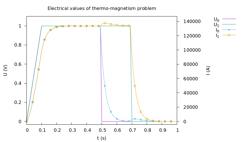
Figure 1. Intensities \(I_i (A)\) and Tensions \(U_i(V)\), caption=

The intensities follow the tensions like for 1-Torus problem with the four step (ramp, trays and cuts). But, we can see little peaks. This peak on one intensity appears when the tension of other conductor is cut. This phenomena is called Electromagnetism Induction.

The Electromagnetism Induction is the production of an electromotive force across an electrical conductor in a changing magnetic field.

With the equation of Maxwell-Faraday :

\[ \nabla \times \mathbf{E} = - \frac{\partial \mathbf{B}}{\partial t}\]

We can see, with time variation of magnetic field \(\mathbf{B}\), we have creation of electrical field. For us case, when we cut the tension for one conductor, we have great time variation of magnetic field thus the other conductor answer by Maxwell-Faraday equation with creation of electrical field and current. When the magnetic field is at zeros, is phenomena disapears.