Test Case of Thermal Dilatation Static in Three Dimensions

1. Introduction

This page presents the test case of Thermal Dilatation implement with CFPDEs with constant temperature without volumic force in static and in three dimensions, solve components by components. This simulation have goal to verify the implementation of thermal dilatation.

2. Run the calculation

The command line to run this case is :

    mpirun -np 16 feelpp_toolbox_coefficientformpdes --config-file=thermal-dilatation.cfg --cfpdes.gmsh.hsize=5e-3

3. Data Files

The case data files are available in Github here :

CFG file - Edit the file
JSON file - Edit the file
GEO file - Edit the file

4. Equation

The domain of resolution is \(\Omega_c^{axis}\) with bounds \(\Gamma_c^{axis}\), \(\Gamma_{D \hspace{0.05cm} elas}^{axis}\) the bound of elastic Dirichlet conditions, \(\Gamma_{N \hspace{0.05cm} elas}^{axis}\) the bound of elastic Neumann conditions such that \(\Gamma_c^{axis} = \Gamma_{D \hspace{0.05cm} elas}^{axis} \cup \Gamma_{N \hspace{0.05cm} elas}^{axis}\).

Differential Formulation of Elasticity Equation in Stationary Case

\[\text{(Static Elasticity)} \left\{ \begin{matrix} - \nabla \cdot \bar{\bar{\sigma}} = \mathbf{F} & \text{on } \Omega_c & \text{(Static Elas-1)} \\ \mathbf{u} = \mathbf{u_0} & \text{on } \Gamma_{D \hspace{0.05cm} elas} & \text{(D elas)} \\ \bar{\bar{\sigma}} \cdot \mathbf{n} = g_N & \text{on } \Gamma_{N \hspace{0.05cm} elas} & \text{(N elas)} \\ \bar{\bar{\sigma}} \cdot \mathbf{n} + k \, \mathbf{u} = g_R & \text{on } \Gamma_{R \hspace{0.05cm} elas} & \text{(R elas)} \end{matrix} \right.\]

With :

Displacement \(\mathbf{u} = \begin{pmatrix} u_x \\ u_y \\ u_z \end{pmatrix}\)
Stress Tensor : \(\bar{\bar{\sigma}}\)
Stiffness tensor : \(k\)
Volumic Forces : \(\mathbf{F}\)

And notations :

Divergence of tensor : \(\nabla \cdot \bar{\bar{\sigma}} = \begin{pmatrix} \nabla \cdot \bar{\bar{\sigma}}_{x,:} \\ \nabla \cdot \bar{\bar{\sigma}}_{y,:} \\ \nabla \cdot \bar{\bar{\sigma}}_{z,:} \end{pmatrix} = \begin{pmatrix} \frac{\partial \bar{\bar{\sigma}}_{xx}}{\partial x} + \frac{\partial \bar{\bar{\sigma}}_{xy}}{\partial y} + \frac{\partial \bar{\bar{\sigma}}_{xz}}{\partial z} \\ \frac{\partial \bar{\bar{\sigma}}_{yx}}{\partial x} + \frac{\partial \bar{\bar{\sigma}}_{yy}}{\partial y} + \frac{\partial \bar{\bar{\sigma}}_{yz}}{\partial z} \\ \frac{\partial \bar{\bar{\sigma}}_{zx}}{\partial x} + \frac{\partial \bar{\bar{\sigma}}_{zy}}{\partial y} + \frac{\partial \bar{\bar{\sigma}}_{zz}}{\partial z} \end{pmatrix}\)
Scalar produce of tensor : \(\bar{\bar{\sigma}} \cdot \mathbf{n} = \begin{pmatrix} \bar{\bar{\sigma}}_{x,:} \cdot \mathbf{n} \\ \bar{\bar{\sigma}}_{y,:} \cdot \mathbf{n} \\ \bar{\bar{\sigma}}_{z,:} \cdot \mathbf{n} \end{pmatrix} = \begin{pmatrix} \bar{\bar{\sigma}}_{xx} \, n_x + \bar{\bar{\sigma}}_{xy} \, n_y + \bar{\bar{\sigma}}_{xz} \, n_z \\ \bar{\bar{\sigma}}_{yx} \, n_x + \bar{\bar{\sigma}}_{yy} \, n_y + \bar{\bar{\sigma}}_{yz} \, n_z \\ \bar{\bar{\sigma}}_{zx} \, n_x + \bar{\bar{\sigma}}_{zy} \, n_y + \bar{\bar{\sigma}}_{zz} \, n_z \end{pmatrix}\)

5. Geometry

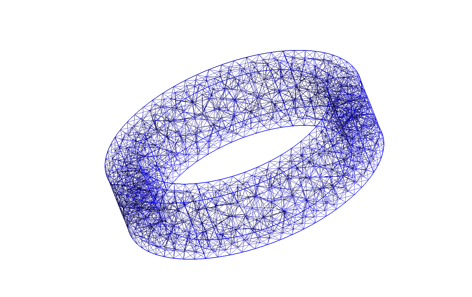
The geometry is a torus of the conductor in cartesian coordinates \((x,y,z)\) or rectangle in axisymmetric coordinates \((r,z)\), surrounded by air.

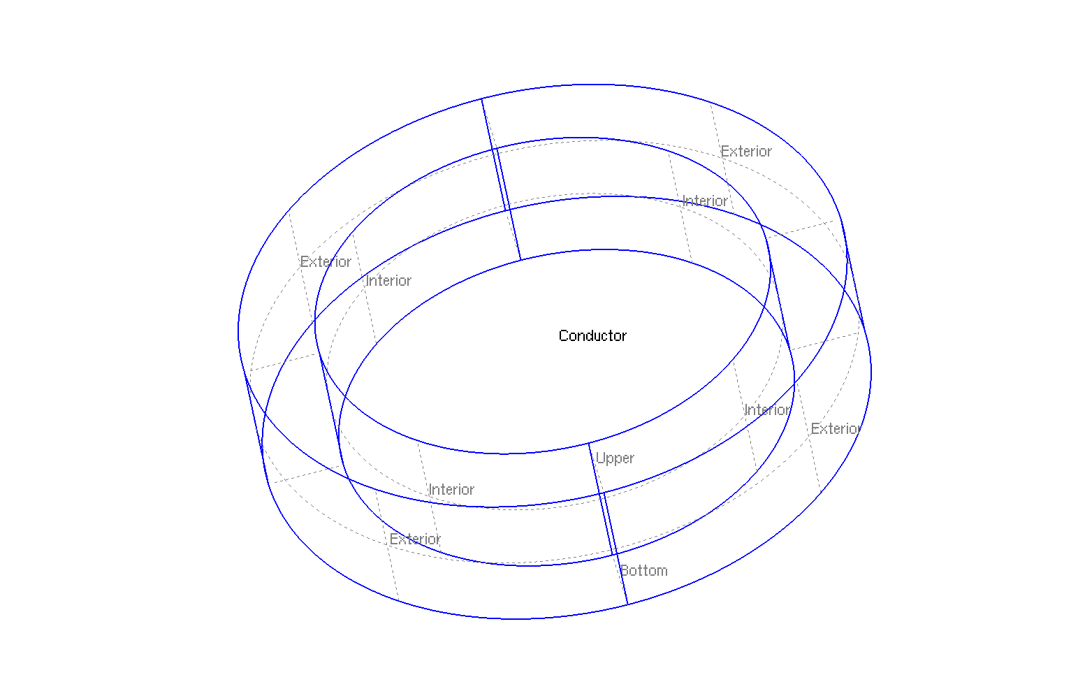
Geometry

The geometrical domains are :

Conductor : the torus is composed by conductor material
- Interior : interior surface of conductor ring
- Exterior : exterior surface of conductor ring
- Upper : upper of conductor ring
- Bottom : bottom of conductor ring
Air : the air surround Conductor
- zAxis : a bound of Air, correspond to \(Oz\) axis (\(\{(z,r), \, z=0 \}\))
- infty : the rest of bound of Air

Symbol

Description

value

unit

\(r_{int}\)

interior radius of torus

\(75e-3\)

\(r_{ext}\)

exterior radius of torus

\(100.2e-3\)

\(z_1\)

half-height of torus

\(25e-3\)

6. Boundary Conditions

We impose the boundary conditions :

Strong Dirichlet : \(\mathbf{u} = 0\) on Upper and Bottom. The Dirichlet condition represents the embedding of mechanical part.
Neumann : \(\bar{\bar{\sigma}} \cdot \mathbf{n} = 0\) on Interior and Exterior. The Neumann condition represents the freedom of displacement.

On JSON file, the boundary conditions are writed :

Boundary conditions on JSON file

    "BoundaryConditions":
    {
        "elastic":
        {
            "Dirichlet":
            {
                "Bottom":
                {
                    "expr":"{0,0,0}"
                },
                "Upper":
                {
                    "expr":"{0,0,0}"
                }
            }
        }
    }

7. Weak Formulation

We obtain :

Weak Formulation of Elasticity Equation in Stationnary Case

\[\text{(Weak Static Elasticity)} \\ \left\{ \begin{matrix} \int_{\Omega_c}{ \bar{\bar{\sigma}}_{xx} \, \frac{\partial \xi_x}{\partial x} + \bar{\bar{\sigma}}_{xy} \, \frac{\partial \xi_x}{\partial y} + \bar{\bar{\sigma}}_{xz} \, \frac{\partial \xi_x}{\partial z} + \bar{\bar{\sigma}}_{yx} \, \frac{\partial \xi_y}{\partial x} + \bar{\bar{\sigma}}_{yy} \, \frac{\partial \xi_y}{\partial y} + \bar{\bar{\sigma}}_{yz} \, \frac{\partial \xi_y}{\partial z} + \bar{\bar{\sigma}}_{zx} \, \frac{\partial \xi_z}{\partial x} + \bar{\bar{\sigma}}_{zy} \, \frac{\partial \xi_z}{\partial y} + \bar{\bar{\sigma}}_{zz} \, \frac{\partial \xi_z}{\partial z} } = \int_{\Omega_c}{ F \cdot \mathbf{ξ} } + \int_{\Gamma_{N \hspace{0.05cm} elas}}{ g_N \cdot \mathbf{ξ} } + \int_{\Gamma_{R \hspace{0.05cm} elas}}{ \left( g_R - \left( k \, u \right) \right) \cdot \mathbf{ξ} } \\ \text{for } \mathbf{ξ} = \begin{pmatrix} \xi_x \\ \xi_y \\ \xi_z \end{pmatrix} \in H^1_{u_0}(\Omega_c) \end{matrix} \right.\]

8. Parameters

The parameters of problem are :

Symbol

Description

Value

Unit

\(E\)

Young Modulus

\(2.1e6\)

\(Pa\)

\(v\)

Poisson’s coefficient

\(0.33\)

\(dimensionless\)

\(\lambda\)

Lame’s coefficient

\(\frac{E \, v}{(1-2v)(1+v)}\)

\(Pa\)

\(\mu\)

Lame’s coefficient

\(\frac{E}{2 (1+v)}\)

\(Pa\)

\(T\)

temperature

\(293\)

\(K\)

\(T_0\)

rest temperature

\(303\)

\(K\)

On JSON file, the parmeters are writed :

Parameters on JSON file

    "Parameters": {
        "E": 2.1e6,
        "nu": 0.33,
        "mu": "E/(2*(1+nu)):E:nu",
        "lambda":"E*nu/((1+nu)*(1-2*nu)):E:nu",
        "T0":293,
        "T":303,
        "alpha_T":"17e-6",
        "sigma_T":"-E/(1-2*nu)*alpha_T*(T-T0):E:nu:alpha_T:T:T0"
    }

9. Coefficient Form PDEs

We use the application Coefficient Form PDEs. The coefficient associate to Weak Formulation are :

Coefficient

Description

Expression

\(c\)

\(\mu\)

\(\mathbf{γ}\)

conservative flux source term

\(\begin{pmatrix} -\lambda \left( \frac{\partial u_x}{\partial x} + \frac{\partial u_y}{\partial y} + \frac{\partial_z}{\partial z} \right) - \sigma_T - \mu \frac{\partial u_x}{\partial x} & -\mu \left( \frac{\partial u_x}{\partial y} + \frac{\partial u_y}{\partial x} \right) & -\mu \left( \frac{\partial u_x}{\partial z} + \frac{\partial u_z}{\partial x} \right) \\ -\mu \left( \frac{\partial u_x}{\partial y} + \frac{\partial u_y}{\partial x} \right) & -\lambda \left( \frac{\partial u_x}{\partial x} + \frac{\partial u_y}{\partial y} + \frac{\partial_z}{\partial z} \right) - \sigma_T - \mu \frac{\partial u_y}{\partial y} & -\mu \left( \frac{\partial u_y}{\partial z} + \frac{\partial u_z}{\partial y} \right) \\ -\mu \left( \frac{\partial u_x}{\partial z} + \frac{\partial u_z}{\partial x} \right) & -\mu \left( \frac{\partial u_y}{\partial z} + \frac{\partial u_z}{\partial y} \right) & -\lambda \left( \frac{\partial u_x}{\partial x} + \frac{\partial u_y}{\partial y} + \frac{\partial_z}{\partial z} \right) - \sigma_T - \mu \frac{\partial u_z}{\partial z} \end{pmatrix}\)

On JSON file, the coefficients are writed :

CFPDEs coefficients on JSON file

    "Materials":
    {
        "Omega":
        {
            "elastic_c": "mu:mu",
            "elastic_gamma":"{-lambda*(elastic_grad_u_00+elastic_grad_u_11+elastic_grad_u_22) - sigma_T - mu*elastic_grad_u_00,-mu*elastic_grad_u_10,-mu*elastic_grad_u_20, -mu*elastic_grad_u_01,-lambda*(elastic_grad_u_00+elastic_grad_u_11+elastic_grad_u_22) - sigma_T - mu*elastic_grad_u_11,-mu*elastic_grad_u_21, -mu*elastic_grad_u_02,-mu*elastic_grad_u_12,-lambda*(elastic_grad_u_00+elastic_grad_u_11+elastic_grad_u_22) - sigma_T - mu*elastic_grad_u_22}:lambda:mu:elastic_grad_u_00:elastic_grad_u_01:elastic_grad_u_10:elastic_grad_u_11:elastic_grad_u_20:elastic_grad_u_21:elastic_grad_u_22:elastic_grad_u_02:elastic_grad_u_12:sigma_T",

            "sigma_xx":"(lambda+2*mu)*elastic_grad_u_00+lambda*elastic_grad_u_11+lambda*elastic_grad_u_22+sigma_T:lambda:mu:elastic_grad_u_00:elastic_grad_u_11:elastic_grad_u_22:sigma_T",
            "sigma_yy":"lambda*elastic_grad_u_00+(lambda+2*mu)*elastic_grad_u_11+lambda*elastic_grad_u_22+sigma_T:lambda:mu:elastic_grad_u_00:elastic_grad_u_11:elastic_grad_u_22:sigma_T",
            "sigma_zz":"lambda*elastic_grad_u_00+lambda*elastic_grad_u_11+(lambda+2*mu)*elastic_grad_u_22+sigma_T:lambda:mu:elastic_grad_u_00:elastic_grad_u_11:elastic_grad_u_22:sigma_T",
            "sigma_xy":"mu*(elastic_grad_u_01+elastic_grad_u_10):mu:elastic_grad_u_01:elastic_grad_u_10",
            "sigma_xz":"mu*(elastic_grad_u_02+elastic_grad_u_20):mu:elastic_grad_u_02:elastic_grad_u_20",
            "sigma_yz":"mu*(elastic_grad_u_12+elastic_grad_u_21):mu:elastic_grad_u_12:elastic_grad_u_21"
        }
    }

10. Numeric Parameters

Mesh size \(10 \, mm\)

Mesh of Geometry

11. Comparison

I run with CATIA (software of conception) the same case. We can compare the result :

Deformation result of dilatation compute with cfpdes : the opaque part is the initial geometry and the transparent part is the geometry after dilatation (with scale=1000)

Deformation result of dilatation compute with catia

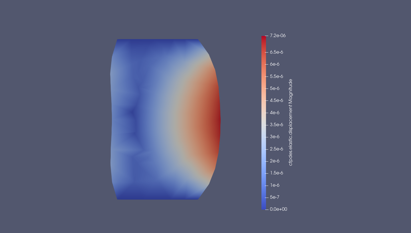
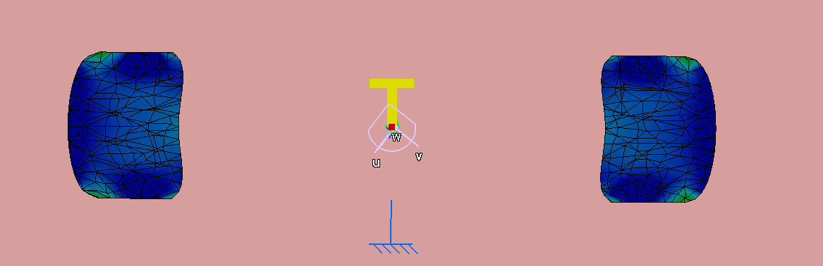
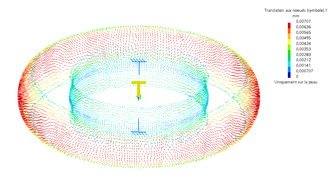
Deformation result of dilatation compute with cfpdes (with scale=1000) : the colours correspond to displacement

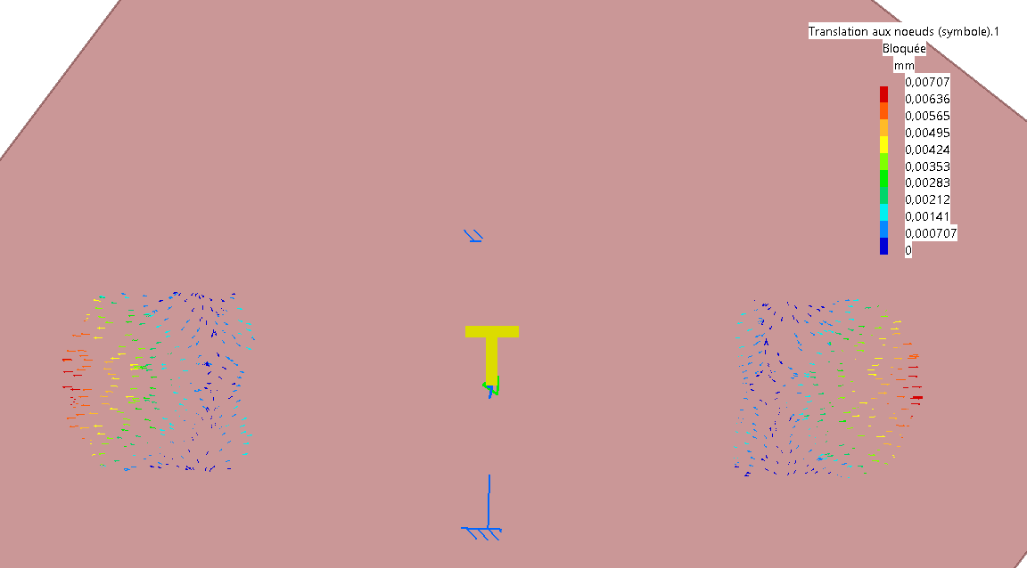
Deformation result of dilatation compute with catia : the colours correspond to displacement

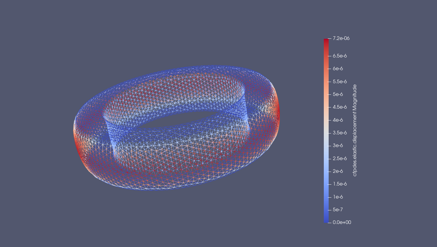
Deformation result of dilatation compute with cfpdes (with scale=1000) : the colours correspond to displacement

Deformation result of dilatation compute with catia (with scale=1000) : the colours correspond to displacement

The comparison isn’t reliable (visual comparison), the result of CFPDEs and CATIA have the form and the same order (near of center-exterior of torus, the displacement is around \(7.2 \, mm\) for the two results).

With comparison with CATIA, we have some confidence in this method.