Test Case of Elasto-Magnetism in Stationary and Axisymmetrical Case

1. Introduction

This page presents the simulation and result of page Elastic Equations with Electromagnetism and Thermic in Axisymmetrical case : Elastic, Thermic and Electromagnetism problem coupled by Thermal Dilatation in stationnary and axisymmetrical case.

2. Run the calculation

The command line to run this case is :

    mpirun -np 16 feelpp_toolbox_coefficientformpdes --config-file=elasto-thermo-mag.cfg --cfpdes.gmsh.hsize=5e-3

To compute with only the Thermal Dilatation, please, put :

        "bool_laplace":0,
        "bool_dilatation":1,

On Parameter function of .json file elasto-thermo-mag.json.

3. Data Files

The case data files are available in Github here :

CFG file - Edit the file
JSON file - Edit the file
GEO file - Edit the file

4. Equation

In this subsection, we couple the equation (Static Elasticity Axis) of Elastic equation and (AV Axis) AV-Formulation in axisymmetrical coordinates.

The domain of resolution of electromagnetism part is \(\Omega^{axis}\) with bounds \(\Gamma^{axis}\), \(\Gamma_D^{axis}\) the bound of Dirichlet conditions and \(\Gamma_N^{axis}\) the bound of Neumann conditions such that \(\Gamma^{axis} = \Gamma_N^{axis} \cup \Gamma_D^{axis}\).

The domain of resolution of elastic part is \(\Omega_c^{axis} \subset \Omega^{axis}\) (and the domain of definition of electrical potential \(V\) and electrical conductivity \(\sigma\)) with bounds \(\Gamma_c^{axis}\), \(\Gamma_{D \hspace{0.05cm} elas}^{axis}\) the bound of Dirichlet conditions and \(\Gamma_{N \hspace{0.05cm} elas}^{axis}\) the bound of Neumann conditions such that \(\Gamma_c^{axis} = \Gamma_{D \hspace{0.05cm} elas}^{axis} \cup \Gamma_{N \hspace{0.05cm} elas}^{axis}\). The domain \(\Omega_c^{axis}\) correspond to the conductor.

Differential Formulation of Elastic Thermic Electromagnetism Equations

\[\small{ \text{(Elasto-Thermo-Elec)} \\ \left\{ \begin{align*} \nabla \times \left( \frac{1}{\mu} \nabla \times \textbf{A} \right) + \sigma(T) \frac{\partial \textbf{A}}{\partial t} + \sigma(T) \nabla V &= 0 & \text{ on } \Omega & \text{(AV-1)} \\ \nabla \cdot \left( \sigma(T) \nabla V + \sigma(T) \frac{\partial \textbf{A}}{\partial t} \right) &= 0 & \text{ on } \Omega_c & \text{(AV-2)} \\ \rho C_p \, \frac{\partial T}{\partial t} - k(T) \Delta T &= \sigma(T) \left( \nabla V + \frac{\partial \mathbf{A}}{\partial t} \right) \cdot \left( \nabla V + \frac{\partial \mathbf{A}}{\partial t} \right) & \text{ on } \Omega_c & \text{(Heat-1)} \\ \frac{\partial \mathbf{p}}{\partial t} - \nabla \cdot \bar{\bar{\sigma}} &= \sigma(T) \, \left( - \nabla V - \frac{d \mathbf{A}}{dt} \right) \times \left( \nabla \times \mathbf{A} \right) & \text{on } \Omega_c & \text{(Elas-1)} \\ \mathbf{A} \times \mathbf{n} &= 0 & \text{ on } \Gamma_D & \text{(AV-D)} \\ \left( \nabla \times \mathbf{A} \right) \times \mathbf{n} &= 0 & \text{ on } \Gamma_N & \text{(AV-N)} \\ \frac{\partial T}{\partial \mathbf{n}} &= 0 & \text{ on } \Gamma_{Nc} & \text{(Heat-N)} \\ - k(T) \, \frac{\partial T}{\partial \mathbf{n}} &= h \, \left( T - T_c \right) & \text{ on } \Gamma_{Rc} & \text{(Heat-R)} \\ \mathbf{u} &= \mathbf{u_0} & \text{on } \Gamma_{D \hspace{0.05cm} elas} & \text{(Elas-D)} \\ \bar{\bar{\sigma}} \cdot \mathbf{n} &= g_N & \text{on } \Gamma_{N \hspace{0.05cm} elas} & \text{(Elas-N)} \\ \end{align*} \right. }\]

With :

Magnetic Potential Field \(\mathbf{A}\)

Temperature \(T\)

Electrical Potential Scalar \(V\)

Thermal Conductivity \(k(T)=\frac{k_0}{1+\alpha (T-T_0)} \frac{T}{T_0}\)

Electrical Conductivity \(\sigma(T)=\frac{\sigma_0}{1+\alpha (T-T_0)}\)

Density \(\rho\)

Thermal Capacity \(C_p\)

Cooling Temperature \(T_c\)

Reference Temperature \(T_0\)

Displacement \(\mathbf{u}\)

Momentum \(\mathbf{p} = \frac{\partial \left( \rho \, \mathbf{u} \right)}{\partial t}\)

Stress Tensor \(\bar{\bar{\sigma}}(\bar{\bar{\epsilon}}) = \bar{\bar{\sigma}}^E(\bar{\bar{\epsilon}}) + \bar{\bar{\sigma}}^T(\bar{\bar{\epsilon}})\)

The tensor of small deformations \(\bar{\bar{\epsilon}} = \frac{1}{2} \left( \nabla \mathbf{u} + \nabla \mathbf{u}^T \right)\)

Lamé’s coefficients : \(\lambda = \frac{E \, v}{(1-2 v) \, (1+v)}\), \(\mu = \frac{E}{2 \, (1+v)}\) with the Young modulus \(E\) and Poisson’s coefficient \(v\)

We don’t care of geometrical deformation which can change the mesh or the density. We suppose the geometry is fixed.

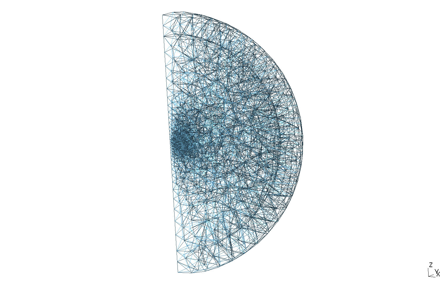
5. Geometry

The geometry is a quart-torus of the conductor in cartesian coordinates \((x,y,z)\).

Geometry

Geometry loop on Conductor

The geometrical domains are :

Conductor : the quart-torus is composed by conductor material
- Interior : interior surface of conductor quart-torus
- Exterior : exterior surface of conductor quart-torus
- Upper : upper of conductor quart-torus
- Bottom : bottom of conductor quart-torus
- V0 : the first bound of quart-torus
- V1 : the second bound of quart-torus
Air : the air surround Conductor
- Infty : the surface of Air at the infty
- OXOZ : the \(O_{xz}\) plan
- OYOZ : the \(O_{yz}\) plan

Symbol

Description

value

unit

\(r_{int}\)

interior radius of quart-torus

\(75e-3\)

\(r_{ext}\)

exterior radius of quart-torus

\(100.2e-3\)

\(z_1\)

half-height of torus

\(300e-3\)

\(r_{inf1}\)

radius of first of Air

\(6*r_{ext}\)

\(r_{inf2}\)

radius of Infty

\(1.2*r_{inf1}\)

6. Boundary Conditions

We impose the boundary conditions :

For Electrical equation of unknow electric potential \(V\) :
- On V0 : \(V = 0\)
- On V1 : \(V = \frac{1}{4} \left\{ \begin{matrix} t \text{ on } 0s \leq t < 1s \\ 1 \text{ on } 1s \leq t < 20s \\ t \text{ on } 20s \leq t \end{matrix} \right.\)
For Magnetic equation of unknow magnetic potential field \(\mathbf{A}\) :
- On OXOZ and V0 : \(A_x = A_z = 0\), we want \(\mathbf{A}\) orthogonal to OXOZ and V0
- On OYOZ and V1 : \(A_y = A_z = 0\), we want \(\mathbf{A}\) orthogonal to OYOZ and V1
- Infty : We approximate the problem, Infty is the physical infty thus \(\mathbf{B}=0\) at Infty thus \(\mathbf{A} = 0\).
For Heat equation of unknow \(T\) :
- On V0, V1, Upper and Bottom, we put Neumann condition \(\frac{\partial T}{\partial \mathbf{n}} = 0\)
- On Interior and Exterior, we put Robin condition \(k \frac{\partial T}{\partial \mathbf{n}} = h \, \left( T - T_c \right)\). It represents the cooling by water.
For Elastic equation of unknow displacement \(u\) :
- On Upper and Bottom, we put Strong Dirichlet condition : \(\mathbf{u} = 0\). The Dirichlet condition represents the embedding of mechanical part.
- On Interior and Exterior, we put Neumann condition : \(\bar{\bar{\sigma}} \cdot \mathbf{n} = 0\). The Neumann condition represents the freedom of displacement.
- On V_0, we put Component Strong Dirichlet : \(u_y = 0\).
- On V_1, we put Component Strong Dirichlet : \(u_x = 0\).

The two Component Strong Dirichlet for Elastic equation represents the fact that the quart of torus is the simplification of a complete torus and because the problem is axisymmetric, the displacement must be on \(O_{rz}\) plan (here it’s \(O_{xz}\) for V0 and \(O_{yz}\) for V1).

On JSON file, the boundary conditions are writed :

Boundary conditions on JSON file

    "BoundaryConditions":
    {
        "magnetic":
        {
            "Dirichlet":
            {
                "Infty":
                {
                    "expr":"{0,0,0}"
                }
            },
            "Dirichlet_x":
            {
                "magdirx":
                {
                    "markers":["V0","OXOZ"],
                    "expr":0
                }
            },
            "Dirichlet_y":
            {
                "magdiry":
                {
                    "markers":["V1","OYOZ"],
                    "expr":0
                }
            },
            "Dirichlet_z":
            {
                "magdirz":
                {
                    "markers":["V0","OXOZ","V1","OYOZ"],
                    "expr":0
                }
            }
        },
        "electric":
        {
            "Dirichlet":
            {
                "V0":
                {
                    "expr":"V0:V0"
                },
                "V1":
                {
                    "expr":"V1:V1"
                }
            }
        },
        "heat":
        {
            "Robin":
            {
                "Interior":
                {
                    "expr1":"h:h",
                    "expr2":"h*T_c:h:T_c"
                },
                "Exterior":
                {
                    "expr1":"h:h",
                    "expr2":"h*T_c:h:T_c"
                }
            }
        },
        "elastic":
        {
            "Dirichlet":
            {
                "V0":
                {
                    "expr":"{0,0,0}"
                },
                "V1":
                {
                    "expr":"{0,0,0}"
                }
            },
            "Dirichlet_x":
            {
                "V1":
                {
                    "expr":0
                }
            },
            "Dirichlet_y":
            {
                "V0":
                {
                    "expr":0
                }
            }
        }
    }

7. Weak Formulation

We obtain :

Weak Formulation of Elastic Thermic Electromagnetism Equations in Stationnary Case Vectorial

\[\tiny{ \text{(Weak Elas-Heat-AV Static)} \\ \begin{eqnarray*} \int_{\Omega}{\frac{1}{\mu} (\nabla \times \textbf{A}) \cdot (\nabla \times \mathbf{ϕ})} + \int_{\Omega_c}{ \sigma \nabla V \cdot \mathbf{ϕ} } + \int_{\Omega}{ \sigma \frac{d \mathbf{A}}{d t} \cdot \mathbf{ϕ} } &=& 0 &\text{(Weak AV-1)} \\ \int_{\Omega_c}{\sigma (\nabla V + \frac{d \mathbf{A}}{d t}) \cdot \nabla \mathbf{\psi}} &=& 0 & \text{(Weak AV-2)} \\ \int_{\Omega_c}{ k \, \nabla T \cdot \nabla \eta } + \int_{\Gamma_R}{ h \, T \, \eta } &=& \int_{\Omega_c}{ Q \, \eta } + \int_{\Gamma_R}{ h \, T_c \, \eta } & \text{(Weak Heat Axis)} \\ \int_{\Omega_c}{ \bar{\bar{\sigma}}_{xx} \, \frac{\partial \xi_x}{\partial x} + \bar{\bar{\sigma}}_{xy} \, \frac{\partial \xi_x}{\partial y} + \bar{\bar{\sigma}}_{xz} \, \frac{\partial \xi_x}{\partial z} + \bar{\bar{\sigma}}_{yx} \, \frac{\partial \xi_y}{\partial x} + \bar{\bar{\sigma}}_{yy} \, \frac{\partial \xi_y}{\partial y} + \bar{\bar{\sigma}}_{yz} \, \frac{\partial \xi_y}{\partial z} + \bar{\bar{\sigma}}_{zx} \, \frac{\partial \xi_z}{\partial x} + \bar{\bar{\sigma}}_{zy} \, \frac{\partial \xi_z}{\partial y} + \bar{\bar{\sigma}}_{zz} \, \frac{\partial \xi_z}{\partial z} } &=& \int_{\Gamma_{N \hspace{0.05cm} elas}}{ \mathbf{g_N} \cdot \mathbf{ξ} } + \int_{\Gamma_{R \hspace{0.05cm} elas}}{ \left( \mathbf{g_R} - ku \right) \cdot \mathbf{ξ} } & \text{(Weak Elas)} \\ \text{for } \mathbf{ϕ} \in H^1(\Omega)^2, \ \psi \in H^1(\Omega_c) , \ \eta \in H^1(\Omega_c) \ \xi = \begin{pmatrix} \xi_x \\ \xi_y \\ \xi_z \end{pmatrix} \in H^1(\Omega_c)^2 \end{eqnarray*} }\]

8. Parameters

The parameters of problem are :

On Conductor :

Symbol

Description

Value

Unit

\(V_0\)

scalar electrical potential on V0

\(0\)

\(Volt\)

\(V_1\)

scalar electrical potential on V0

\(\frac{1}{4} \times 0.2\)

\(Volt\)

\(\sigma\)

electrical conductivity

\(58e6\)

\(S/m\)

\(\mu=\mu_0\)

magnetic permeability of vacuum

\(4\pi.10^{-7}\)

\(kg.m/A^2/S^2\)

\(k\)

thermal conductivity

\(380\)

\(W/m/K\)

\(C_p\)

thermal capacity

\(380\)

\(J/K/kg\)

\(\rho\)

density

\(10000\)

\(kg/m^3\)

\(h\)

convective coefficient

\(80000\)

\(W/m^2/K\)

\(T_c\)

cooling temperature

\(293\)

\(K\)

\(T_0\)

temperature of reference or rest temperature

\(293\)

\(K\)

\(E\)

Young Modulus

\(2.1e6\)

\(Pa\)

\(\nu\)

Poisson’s coefficient

\(0.33\)

\(dimensionless\)

\(Lame\_\lambda\)

Lame’s coefficient

\(\frac{E \, v}{(1-2v)(1+v)}\)

\(Pa\)

\(Lame\_\mu\)

Lame’s coefficient

\(\frac{E}{2 (1+v)}\)

\(Pa\)

\(\alpha_T\)

linear coefficient of dilatation

\(17e-6\)

\(K^{-1}\)

\(\sigma_T = -\frac{E}{1-2*nu} alpha_T (T-T0)\)

thermal dilatation term

\(\frac{E}{2 (1+v)}\)

\(Pa\)

On Air :

Symbol

Description

Value

Unit

\(\mu=\mu_0\)

magnetic permeability of vacuum

\(4\pi.10^{-7}\)

\(kg \, m / A^2 / S^2\)

On JSON file, the parmeters are writed :

Parameters on JSON file

   "Parameters":
    {
        "bool_laplace":1,
        "bool_dilatation":0,

        "V0":0,
        "V1":"1/4*0.2",

        "h":80000,  // W/m2/K
        "T_c":293,  // K
        "T_i":293,  // K

        // Constants of analytical solve
        "a":1933.10,    // K
        "b":0.40041,    // K
        "rmax":0.0861910719118454,  // m
        "Tmax":364.446  // K
    }

9. Coefficient Form PDEs

We use the application Coefficient Form PDEs. The coefficient associate to Weak Formulation are :

For MQS equation (Weak MQS Axis) :
- On Conductor :
Coefficient

Description

Expression

\(c\)

diffusion coefficient

\(\frac{1}{\mu}\)

\(f\)

source term

\(- \sigma \, \nabla V\)
- On Air :
Coefficient

Description

Expression

\(c\)

diffusion coefficient

\(\frac{1}{\mu}\)
For heat equation, on Conductor (the temperature isn’t computed on Air)

Coefficient

Description

Expression

\(c\)

diffusion coefficient

\(k\)

\(f\)

source term

\(\sigma \Vert \nabla V \Vert\)

For elastic equation, on Conductor (the displacement isn’t computed on Air) :

Coefficient

Description

Expression

\(c\)

diffusion coefficient

\(Lame\_\mu\)

\(\gamma\)

conservative flux source term

\(\begin{pmatrix} - Lame\_\lambda \nabla \cdot \mathbf{u} - Lame\_\mu \frac{\partial u_x}{\partial x} - \sigma_T & -Lame\_\mu \frac{\partial u_y}{\partial x} & -Lame\_\mu \frac{\partial u_z}{\partial x} \\ -Lame\_\mu \frac{\partial u_x}{\partial y} & - Lame\_\lambda \nabla \cdot \mathbf{u} - Lame\_\mu \frac{\partial u_y}{\partial y} - \sigma_T & -Lame\_\mu \frac{\partial u_z}{\partial y} \\ -Lame\_\mu \frac{\partial u_x}{\partial z} & -Lame\_\mu \frac{\partial u_y}{\partial z} & - Lame\_\lambda \nabla \cdot \mathbf{u} - Lame\_\mu \frac{\partial u_z}{\partial z} - \sigma_T \end{pmatrix}\)

\(f\)

source term

\(\begin{pmatrix} 0 \\ 0 \\ 0 \end{pmatrix}\)

On JSON file, the coefficients are writed :

CFPDEs coefficients on JSON file

    "Materials":
    {
        "Conductor":
        {
            // Electric Part
            "sigma":58e6,       // S.m-1
            "mu":"4*pi*1e-7",   // kg.m/A2/S2
            "magnetic_c":"1/mu:mu",
            "magnetic_f":"{-sigma*electric_grad_V_0,-sigma*electric_grad_V_1,-sigma*electric_grad_V_2}:sigma:electric_grad_V_0:electric_grad_V_1:electric_grad_V_2",

            "electric_c":"sigma:sigma",

            // Thermic Part
            "k":380,        // W/m/K
            "heat_c":"k:k",
            "heat_f":"sigma*(electric_grad_V_0*electric_grad_V_0+electric_grad_V_1*electric_grad_V_1+electric_grad_V_2*electric_grad_V_2):sigma:electric_grad_V_0:electric_grad_V_1:electric_grad_V_2",

            // Elastic Part
            "E": 2.1e6,
            "nu": 0.33,
            "Lame_lambda":"E*nu/((1+nu)*(1-2*nu)):E:nu",
            "Lame_mu": "E/(2*(1+nu)):E:nu",

            "alpha_T":"17e-6",
            "sigma_T":"-E/(1-2*nu)*alpha_T*(T-T0):E:nu:alpha_T:T:T0",

            "F_laplace":"{-sigma*electric_grad_V_1*(magnetic_grad_A_10-magnetic_grad_A_01)+sigma*electric_grad_V_2*(-magnetic_grad_A_20+magnetic_grad_A_02),sigma*electric_grad_V_0*(magnetic_grad_A_10-magnetic_grad_A_01)-sigma*electric_grad_V_2*(magnetic_grad_A_21-magnetic_grad_A_12),-sigma*electric_grad_V_0*(-magnetic_grad_A_20+magnetic_grad_A_02)+sigma*electric_grad_V_1*(magnetic_grad_A_21-magnetic_grad_A_12)}:sigma:electric_grad_V_0:electric_grad_V_1:electric_grad_V_2:magnetic_grad_A_10:magnetic_grad_A_01:magnetic_grad_A_20:magnetic_grad_A_02:magnetic_grad_A_12:magnetic_grad_A_21",

            "elastic_c": "Lame_mu:Lame_mu",
            "elastic_gamma":"{-Lame_lambda*(elastic_div_u) - Lame_mu*elastic_grad_u_00 - bool_dilatation*sigma_T,-Lame_mu*elastic_grad_u_10,-Lame_mu*elastic_grad_u_20, -Lame_mu*elastic_grad_u_01,-Lame_lambda*(elastic_div_u) - Lame_mu*elastic_grad_u_11 - bool_dilatation*sigma_T,-Lame_mu*elastic_grad_u_21, -Lame_mu*elastic_grad_u_02,-Lame_mu*elastic_grad_u_12,-Lame_lambda*(elastic_div_u) - Lame_mu*elastic_grad_u_22 - bool_dilatation*sigma_T}:bool_dilatation:sigma_T:Lame_lambda:Lame_mu:elastic_div_u:elastic_grad_u_00:elastic_grad_u_01:elastic_grad_u_10:elastic_grad_u_11:elastic_grad_u_20:elastic_grad_u_21:elastic_grad_u_22:elastic_grad_u_02:elastic_grad_u_12",
            "elastic_f":"{bool_laplace*F_laplace_0,bool_laplace*F_laplace_1,bool_laplace*F_laplace_2}:bool_laplace:F_laplace_0:F_laplace_1:F_laplace_2",

            "sigma_xx":"(Lame_lambda+2*Lame_mu)*elastic_grad_u_00+Lame_lambda*elastic_grad_u_11+Lame_lambda*elastic_grad_u_22+bool_dilatation*sigma_T:bool_dilatation:Lame_lambda:Lame_mu:elastic_grad_u_00:elastic_grad_u_11:elastic_grad_u_22:sigma_T",
            "sigma_yy":"Lame_lambda*elastic_grad_u_00+(Lame_lambda+2*Lame_mu)*elastic_grad_u_11+Lame_lambda*elastic_grad_u_22+bool_dilatation*sigma_T:bool_dilatation:Lame_lambda:Lame_mu:elastic_grad_u_00:elastic_grad_u_11:elastic_grad_u_22:sigma_T",
            "sigma_zz":"Lame_lambda*elastic_grad_u_00+Lame_lambda*elastic_grad_u_11+(Lame_lambda+2*Lame_mu)*elastic_grad_u_22+bool_dilatation*sigma_T:bool_dilatation:Lame_lambda:Lame_mu:elastic_grad_u_00:elastic_grad_u_11:elastic_grad_u_22:sigma_T",
            "sigma_xy":"Lame_mu*(elastic_grad_u_01+elastic_grad_u_10):Lame_mu:elastic_grad_u_01:elastic_grad_u_10",
            "sigma_xz":"Lame_mu*(elastic_grad_u_02+elastic_grad_u_20):Lame_mu:elastic_grad_u_02:elastic_grad_u_20",
            "sigma_yz":"Lame_mu*(elastic_grad_u_12+elastic_grad_u_21):Lame_mu:elastic_grad_u_12:elastic_grad_u_21"
        }

10. Numeric Parameters

Mesh size :
- Interior of torus : \(0.01 m\)
- Far from the torus : \(0.2 m\)
Element Type : I run the simulation in \(P_2\) elements.

Mesh of Geometry

11. Result

I have no time to export the data.