Test case of Thermo-Magnetism with Linear Coefficients in Axisymmetrical case
1. Introduction
This page presents the simulation of electromagnetism in A-V Formulation coupled with thermic problem on geometry of torus in transient case in axisymmetrical case with CFPDEs application.
2. Run the calculation
The command line to run this case is :
mpirun -np 4 feelpp_toolbox_coefficientformpdes --config-file=thermo-mag.cfg --cfpdes.gmsh.hsize=1e-3
To run the case with adaptative time-step :
sh feelpp_adaptative.sh
3. Data Files
The case data files are available in Github here :
-
CFG file - Edit the file
-
JSON file - Edit the file
-
GEO file - Edit the file
-
SH script for adaptative time-step - Edit the file
4. Equation
-
With \(\Phi = r \, A_{\theta}\)
5. Geometry
The geometry is a torus of the conductor in cartesian coordinates \((x,y,z)\) or rectangle in axisymmetric coordinates \((r,z)\), surrounded by air.
.png)
Geometry in axisymmetrical cut loop on Conductor
|
.png)
Geometry in axisymmetrical cut
|
.png)
Geometry in three dimensions
|
.png)
Geometry in three dimensions cut loop on Conductor
|
The geometrical domains are :
-
Conductor: the torus is composed by conductor material-
Interior: interior surface of conductor ring -
Exterior: exterior surface of conductor ring -
Upper: upper of conductor ring -
Bottom: bottom of conductor ring
-
-
Air: the air surroundConductor-
zAxis: a bound ofAir, correspond to \(Oz\) axis (\(\{(z,r), \, z=0 \}\)) -
infty: the rest of bound ofAir
-
Symbol |
Description |
value |
unit |
\(r_{int}\) |
interior radius of torus |
\(75e-3\) |
m |
\(r_{ext}\) |
exterior radius of torus |
\(100.2e-3\) |
m |
\(z_1\) |
half-height of torus |
\(25e-3\) |
m |
6. Initial/Boundary Conditions
We impose the boundary conditions :
-
Dirichlet :
-
On
zAxis: \(\Phi = 0\) (\(A_{\theta} = 0\) by symetric argument) -
On
infty: \(\Phi = 0\) (\(A_{\theta} = 0\) we consider the bound of resolution like infty for magnetic field)
-
-
Neumann : \(\frac{\partial T}{\partial \mathbf{n}} = 0\) on
InteriorandExterior -
Robin : \(-k \, \frac{\partial T}{\partial \mathbf{n}} = h \, \left( T - T_c \right)\) on
UpperandBottom
We initialize :
-
On
Conductor\(\Phi(t=0,r,z) = 0\) (\(A_{\theta}(t=0,r,z) = 0\)) and \(T(t=0,r,z) = T_i\) -
On
Air\(\Phi(t=0,r,z) = 0\) (\(A_{\theta}(t=0,r,z) = 0\))
On JSON file, the boundary conditions are writed :
    "BoundaryConditions":
    {
        "magnetic":
        {
            "Dirichlet":
            {
                "ZAxis":
                {
                    "expr":"0"
                },
                "Infty":
                {
                    "expr":"0"
                }
            }
        },
        "heat":
        {
            "Robin":
            {
                "Interior":
                {
                    "expr1":"h*x:h:x",
                    "expr2":"h*T_c*x:h:T_c:x"
                },
                "Exterior":
                {
                    "expr1":"h*x:h:x",
                    "expr2":"h*T_c*x:h:T_c:x"
                }
            }
        }
    }
On JSON file, the intial conditions are writed : .Initial conditions on JSON file
    "InitialConditions":
    {
        "temperature":
        {
            "Expression":
            {
                "myic":
                {
                    "markers":"Conductor",
                    "expr":"T_i:T_i"
                }
            }
        }
    }
7. Weak Formulation
We obtain :
With \(\tilde{\nabla} = \begin{pmatrix} \frac{\partial}{\partial r} \\ \frac{\partial}{\partial z} \end{pmatrix}\)
8. Parameters
The parameters of problem are :
-
On
Conductor:
Symbol |
Description |
Value |
Unit |
\(V\) |
scalar electrical potential |
\( U \, \frac{\theta}{2\pi}\) |
\(Volt\) |
\(U\) |
electrical potential |
\(\left\{ \begin{matrix} t \text{ on } 0s \leq t \leq 1s \\ 1 \text{ on } 1s \leq t \leq 20s \\ 0 \text{ on } 20s \leq t \leq 22s \end{matrix} \right.\) |
\(Volt\) |
\(\sigma\) |
electrical conductivity |
\(4.8e7\) |
\(S/m\) |
\(\mu=\mu_0\) |
magnetic permeability of vacuum |
\(4\pi.10^{-7}\) |
\(kg \, m / A^2 / S^2\) |
\(k\) |
thermal conductivity |
\(380\) |
\(W/m/K\) |
\(C_p\) |
thermal capacity |
\(380\) |
\(J/K/kg\) |
\(\rho\) |
density |
\(10000\) |
\(kg/m^3\) |
\(h\) |
convective coefficient |
\(80000\) |
\(W/m^2/K\) |
\(T_c\) |
cooling temperature |
\(293\) |
\(K\) |
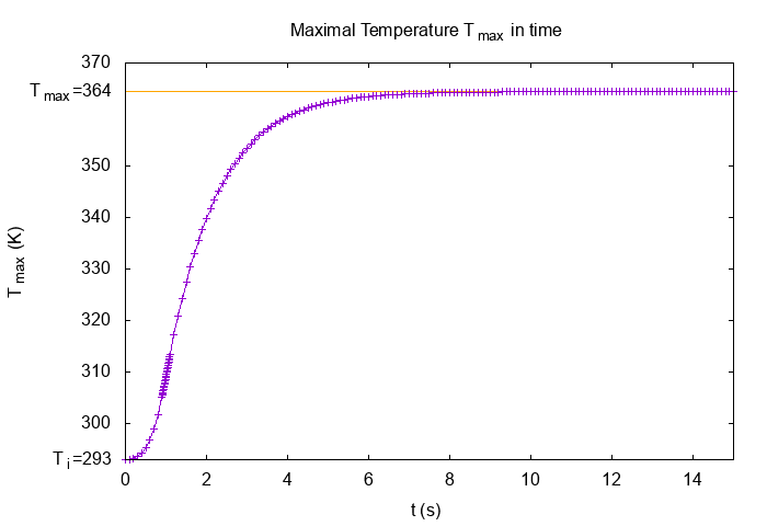
\(T_i\) |
initial temperature |
\(293\) |
\(K\) |
-
On
Air:
Symbol |
Description |
Value |
Unit |
\(\mu=\mu_0\) |
magnetic permeability of vacuum |
\(4\pi.10^{-7}\) |
\(kg \, m / A^2 / S^2\) |
On JSON file, the parmeters are writed :
"Parameters":
{
"h":80000, // W*m-2*K-1
"T_c":293, // K
"T_i":293, // K
"U":"t/1.*(t<1.)+(t<20.)*(t>1.):t", // Volt
// Constants of analytical solve
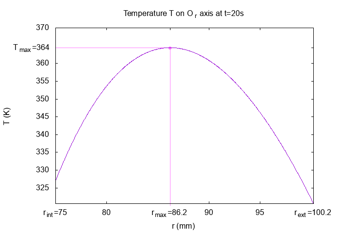
"a":1933.10, // K
"b":0.40041, // K
"rmax":0.0861910719118454, // m
"Tmax":364.446 // K
}
9. Coefficient Form PDEs
We use the application Coefficient Form PDEs. The coefficient associate to Weak Formulation are :
-
For MQS equation (Weak MQS Axis) :
-
On
Conductor:
Coefficient
Description
Expression
\(d\)
damping or mass coefficient
\(\sigma\)
\(c\)
diffusion coefficient
\(\frac{r}{\mu}\)
\(\beta\)
convection coefficient
\(\begin{pmatrix} \frac{2}{\mu} \\ 0 \end{pmatrix}\)
\(f\)
source term
\(- \sigma \frac{U}{2\pi} \, r\)
-
On
Air:
Coefficient
Description
Expression
\(c\)
diffusion coefficient
\(\frac{r}{\mu}\)
-
-
For heat equation (Weak Heat Axis), on
Conductor(the temperature isn’t computed onAir) :Coefficient
Description
Expression
\(d\)
damping or mass coefficient
\(\rho \, C_p\)
\(c\)
diffusion coefficient
\(k\)
\(f\)
source term
\(\sigma \left( \frac{U}{2\pi} \right)^2 \frac{1}{r}\)
On JSON file, the coefficients are writed :
    "Materials":
    {
        "Conductor":
        {
            "sigma":58e+6,  // S.m-1
            "mu":"4*pi*1e-7",   // kg.m/A2/S2
	        "magnetic_c":"x/mu:x:mu",
            "magnetic_beta":"{2/mu,0}:mu",
            "magnetic_f":"-sigma*U/2/pi*x:sigma:U:x",
            "magnetic_d":"sigma*x:x:sigma",

            "k":380,        // W/m/K
            "rho":10000,    // kg/m3
            "Cp":380,       // J/K/kg
            "heat_c":"k*x:k:x",
            "heat_f":"sigma*(U/(2*pi)+magnetic_dphi_dt)*(U/(2*pi)+magnetic_dphi_dt)/x:sigma:U:magnetic_dphi_dt:x",
            "heat_d":"rho*Cp*x:rho:Cp:x"
        },
        "Air":
        {
            "physics":"magnetic",
            "mu":"4*pi*1e-7",   // kg.m/A2/s2
            "magnetic_c":"x/mu:x:mu",
            "magnetic_beta":"{2/mu,0}:mu"
        }
    }
10. Numeric Parameters
This section show the parameters used to compute the simulation.
-
Size of mesh : \(1 \, mm\)
-
Time Parameters :
-
Time step : I use adaptative time step. Near of brutal changement of current, the time step is little, in other case, the time step is big. I put adaptative time step to have good precision near of changement (cut of current at \(t=22s\)) and to not explose the time of compute. The shell script feelpp_adaptative.sh implements that.
\(\Delta_t = \left\{ \begin{matrix} 0.1s \, \text{for} \, 0s<t<0.9s \\ 0.008s \, \text{for} \, 0.9s<t<1.1s \\ 0.1s \, \text{for} \, 1.1s<t<19.9s \\ 0.008s \, \text{for} \, 19.9s<t<20.1s \\ 0.1 \, \text{for} \, 20.1s<t<22s \end{matrix} \right.\)
-
Initial Time : \(0 \, s\)
-
Final Time : \(22 \, s\)
-
-
Element type : \(P2\) for magnetic equation (\(\mathbf{A}\) and \(P1\) heat equation (\(T\))
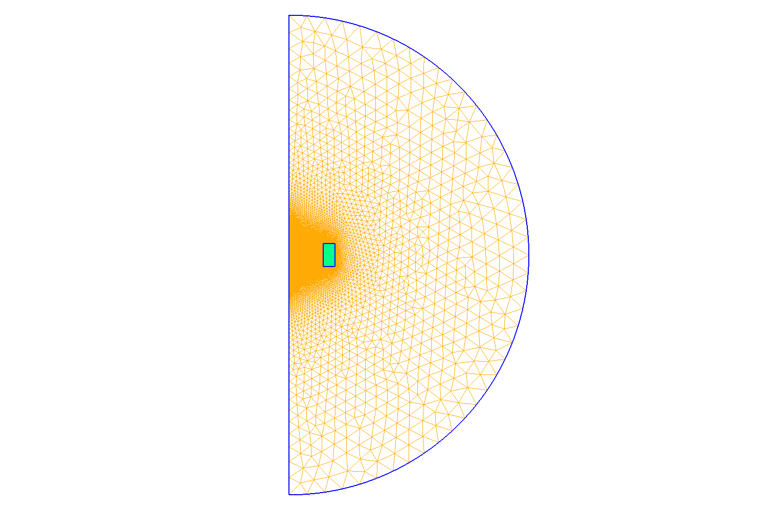
Mesh of Geometry
|
11. Exact solutions
11.1. Intensity
In this subsection, we see the analytical compute of intensity.
We have :
| In stationary case we have \(U = R \, I\). |
And :
-
Resolution of first part (\(0s \leq t \leq 1s\)) :
The homogenous equation \(R \, I_0 + L \, \frac{dI_0}{dt} = 0\) have a solve : \(I_0(t) = e^{-\frac{R}{L}t}\)
We pose \(C(t)\), such that \(I(t) = C(t) \, I_0(t) = C(t) \, e^{-\frac{R}{L}t}\) is solution of equation (Intensity-1).
Thus :
Thus :
-
Resolution of second part (\(1s \leq t \leq 20s\)) :
An evident solution is :
-
Resolution of third part (\(20s \leq t\)) :
An evident solution is :
To conclude, we have :
This solution is compute with python script.
12. Result
The analytical solve of potential magnetic field and magnetic field (the cyan curve on plots) is computed by python3’s module MagnetTools.MagnetTools. The module based on paper : spire.
The analytical solve of intensity (and magnetic field) is computed on python3’s script Edit the file.
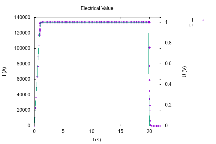
12.1. Intensity
Feelpp compute in post-process, the intensity of circuit :
The intensity verify the equation :
With \(R\) the resistance of torus of conductor and \(L\) the inductance of conductor.
In case of a rectangular cross section \((r_{int},r_{ext}) \times (z_1,z_2)\) torus, we can show that :
We have the value :
Symbol |
Description |
Value |
Unit |
R |
resistance of torus |
\(7.5313 \times 10^{-6}\) |
Ohm |
L |
inductance of torus |
\(1.9204 \times 10^{-7}\) |
Henry |
The exact solution is (see the subsection Intensity for more detail) :
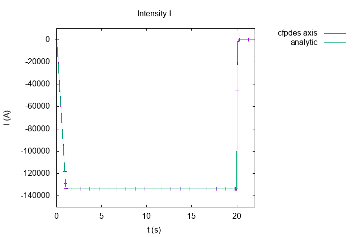
Intensity of current \(I(A)\)
|
In stationary case, we have the Ohm law :
With this relation, we have theorycal intensity : \(I_{th} = \frac{U}{R} = -132779 \, A\). And with numeric solve, we have \(I_{num} = -1.3376228966881469e+05 \, A\), so an error of \(7.4e-3 \, A\).
12.2. Magnetic field \(B_z\)
Recall, with axisymmetric condition :
Thus \(B_z = \frac{1}{r} \frac{\partial \Phi}{\partial r} \).
-
On \(Or\) axis at \(t=20s\)
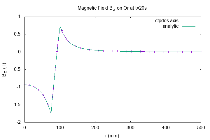
Horizontal Magnetic Field \(B_z(T)\) on Or
|
-
On origin \((0,0,0)\) across the time
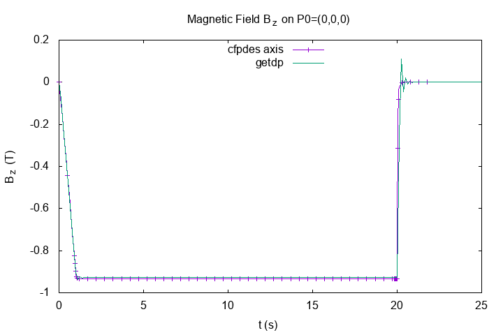
"Horizontal Magnetic Field \(B_z(T)\)
|
-
Magnetic Field across the time :
Horizontal Magnetic Field \(B_z(T)\)
|