SEISM

1. Introduction

The LPSC (Laboratoire de Physique Subatomique & Cosmologie) has developed SEISM, the first and unique confinement structure in the world that allows a closed ECR zone, using advanced magnet technology from LNCMI Grenoble (High Magnetic Field Laboratory).

An ECR zone is a zone of plasma formation.

This page presents the simulation thermo-magnetism problem of SEISM in axisymmetrical case by CoefficientForm PDE’s, an application of LNCMI.

2. Run the calculation

The command line to run this case is :

To generate the mesh :

gmsh -2 -bin Chambre_1.geo

To search the tensions associated to desired intensities :

python3 seism.py

To run the simulation in transient case :

mpirun -np 16 feelpp_toolbox_coefficientformpdes --config-file=seism.cfg

3. Data Files

The case data files are available in Github here :

Linear Case
- PYTHON file - Edit the file
- CFG file - Edit the file
- JSON file - Edit the file
- GEO file - Edit the file

The files of configuration and parameters to simulate the static case and used by python’s script are seism_static.cfg and seism_static.json.

Non Linear Case :
- PYTHON file - Edit the file
- CFG file - Edit the file
- JSON file - Edit the file
- GEO file - Edit the file

The folder seism-detail contains the same files but for an geometry with physical group more detailed.

4. Equation

In this subsection, we retake the coupled equation (AV+Heat Axis) of Heat equation and AV-Formulation in axisymetrical coordinates with new coefficients.

The domain of resolution of electromagnetism part is \(\Omega^{axis}\) with bounds \(\Gamma^{axis}\), \(\Gamma_D^{axis}\) the bound of Dirichlet conditions and \(\Gamma_N^{axis}\) the bound of Neumann conditions such that \(\Gamma^{axis} = \Gamma_N^{axis} \cup \Gamma_D^{axis}\).

The domain of resolution of heat part is \(\Omega_c^{axis} \subset \Omega^{axis}\) (and the domain of definition of electrical potential \(V\) and electrical conductivity \(\sigma\)) with bounds \(\Gamma_c^{axis}\), \(\Gamma_{Dc}^{axis}\) the bound of Dirichlet conditions and \(\Gamma_{Nc}^{axis}\) the bound of Neumann conditions such that \(\Gamma_c^{axis} = \Gamma_{Nc}^{axis} \cup \Gamma_{Dc}^{axis}\).

Differential Formulation in Axisymmetric

\[\text{(AV+Heat Axis)} \left\{ \begin{matrix} \sigma(T) \, \frac{\partial \Phi}{\partial t} - \frac{1}{\mu} \Delta \Phi + \frac{2}{\mu \, r} \frac{\partial \Phi}{\partial r} + \sigma(T) \, \frac{\partial V}{\partial \theta} = 0 & \text{ on } \Omega^{axis} & \text{(AV-1 Axis)} \\ V = \frac{U}{2\pi} \, \theta & \text{ on } \Omega_c^{axis} \\ A_{\theta} = 0 & \text{ on } \Gamma_D^{axis} & \text{(D Axis)} \\ \frac{\partial A_{\theta}}{\partial \mathbf{n}^{axis}} = 0 & \text{ on } \Gamma_N^{axis} & \text{(N Axis)} \\ \rho C_p \, \frac{\partial T}{\partial t} - k(T) \, \Delta T = \sigma \, \left( \frac{1}{r} \, \frac{\partial V}{\partial \theta} + \frac{\partial A_{\theta}}{\partial t} \right)^2 & \text{ on } \Omega_c^{axis} & \text{(Heat Axis)} \\ \frac{\partial T}{\partial \mathbf{n}^{axis}} = 0 & \text{ on } \Gamma_{Nc}^{axis} & \text{(Nc Axis)} \\ - k(T) \, \frac{\partial T}{\partial \mathbf{n}^{axis}} = h \, \left( T - T_c \right) & \text{ on } \Gamma_{Rc}^{axis} & \text{(Rc Axis)} \end{matrix} \right.\]

With :

\(\Phi = r \, A_{\theta}\), with magnetic potential field \(\mathbf{A} = \begin{pmatrix} A_r \\ A_{\theta} \\ A_z \end{pmatrix}_{cyl}\) such that the magnetic field is writed \(\mathbf{B} = \nabla \times \mathbf{A}\)
\(T\) : temperature \((K)\)
\(\sigma\) : electric conductivity \((S/m)\)
\(\mu\) : electric permeability \((kg/A^2/S^2)\)
\(\rho\) : density \((kg/m^3)\)
\(C_p\) : thermal capacity \((J/K/kg)\)
\(k\) : thermal conductivity \((W/m/K)\)
\(U\) : tension \(Volt\)

We run the simulation in two cases :

with Linear coefficients : the electrical conductivity \(\sigma\) and thermal conductivity \(k\) are constant.
with Non-Linear coefficients : the electrical conductivity \(\sigma = \frac{\sigma_0}{1 + \alpha \, \left( T - T_0 \right)}\) and thermal conductivity \(k = \frac{k_0}{1 + \alpha \, \left( T - T_0 \right)} \, \frac{T}{T_0}\) with \(T_0\) temperature of reference, \(sigma_0\) the electrical conductivity of at temperature of reference, \(k_0\) the thermal conductivity at temperature of reference and \(\alpha\) temperature coefficient.

5. Geometry

The axisymmetrical geometry of SEISM is composed by 4 Helix :

Two Helix of Injection
- Helix1 + Helix2 + Helix3 the first helix
- Helix5 the second
Two Helix of Ejection
- Helix4 the first
- Helix6 the second
All Helixi have the bounds :
- RChanneli : the bound of inter-spire
- Rinti : the interior bound of spires
- Rexti : the exterior bound of spires
The Air surrounding the helix
- Air : the exterior air
- AifInf : the interior air
- Axis : \(Oz\) axis
- Infini : the bound of Axis

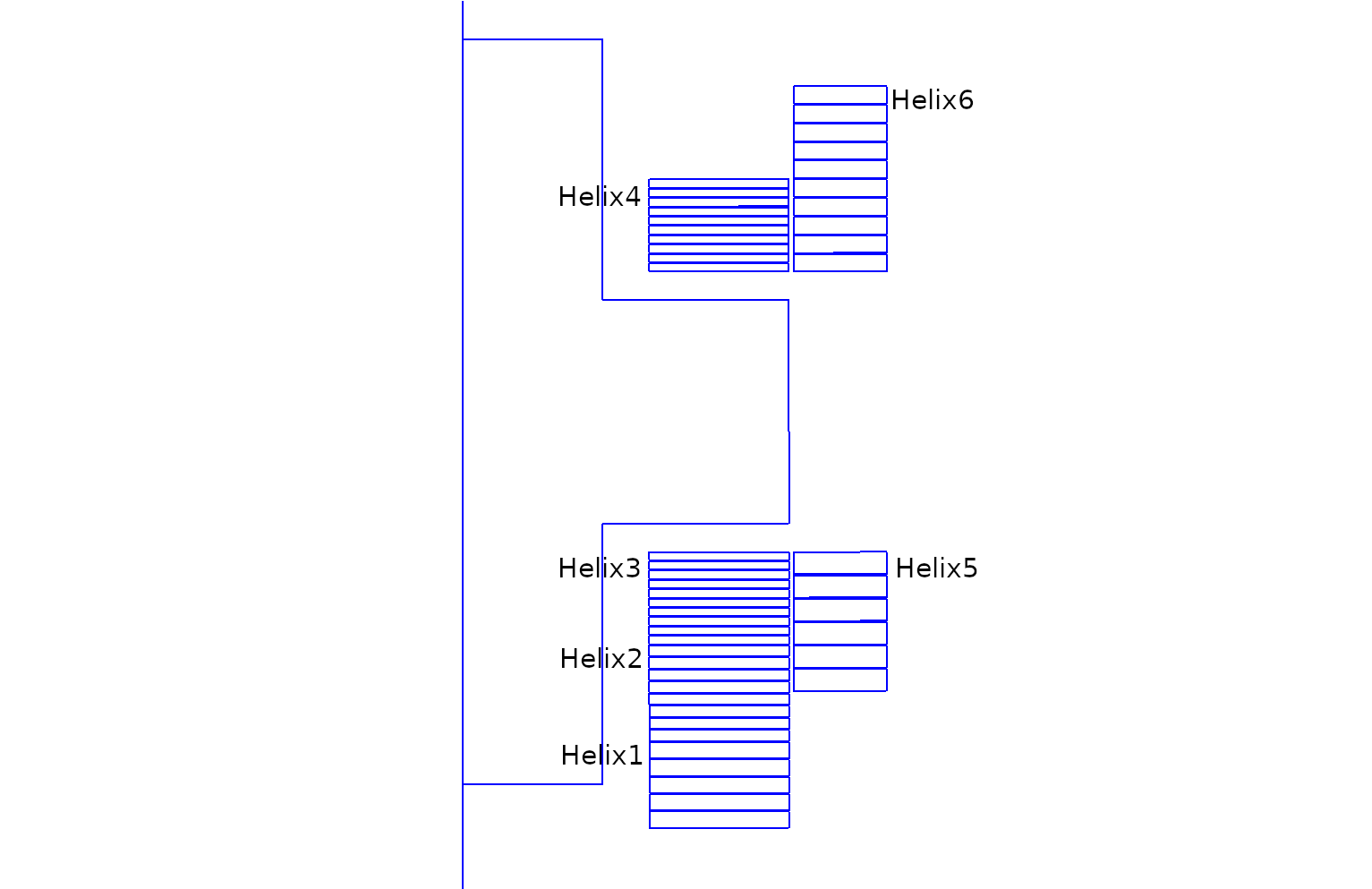
Geometry of SEISM

Geometry of Helix5

The physical groups Helixi is composed by \(n_{spire \, i}\) of half-height \(z_i\), interior radius \(r_{int \, i}\) ans exterior radius \(r_{ext \, i}\) :

Geometrical Parameter

Helix1

Helix2

Helix3

Helix4

Helix5

Helix6

Unit

\(n_{spire}\)

\(z_i\)

\(3.73\)

\(26\)

\(2.0\)

\(5.0\)

\(4.0\)

\(mm\)

\(r_{ext}\)

\(40\)

\(71\)

\(40\)

\(71\)

\(mm\)

\(r_{int}\)

\(70\)

\(91\)

\(70\)

\(91\)

\(mm\)

Symbol

Description

Value

Unit

\(r_{inf}\)

Intermediate radius of Air

\(1.5\)

\(m\)

\(r_{ext}\)

Radius of Boundary of Air

\(3\)

\(m\)

6. Initial/Boundary Conditions

We impose the boundary conditions :

Dirichlet :
- On Axis : \(\Phi = 0\) (\(A_{\theta} = 0\) by symetric argument)
- On Infini : \(\Phi = 0\) (\(A_{\theta} = 0\) we consider the bound of resolution like infty for magnetic field)
Robin :
- \(-k \, \frac{\partial T}{\partial \mathbf{n}} = h_{int} \, \left( T - T_c \right)\) on Rinti
- \(-k \, \frac{\partial T}{\partial \mathbf{n}} = h_{ext} \, \left( T - T_c \right)\) on Rexti
- \(-k \, \frac{\partial T}{\partial \mathbf{n}} = h_{ch} \, \left( T - T_c \right)\) on RChanneli

On JSON file, the boundary conditions are writed :

Boundary conditions on JSON file

    "BoundaryConditions":
    {
        "magnetic":
        {
            "Dirichlet":
            {
                "magdir":
                {
                    "markers":["Axis","Infini"],
                    "expr":"0"
                }
            }
        },
        "heat":
        {
            "Robin":
            {
                "heatrobin_int":
                {
                    "markers":["Rint1","Rint2","Rint3","Rint4","Rint5","Rint6"],
                    "expr1":"h_int*x:h_int:x",
                    "expr2":"h_int*T_c*x:h_int:T_c:x"
                },
                "heatrobin_ext":
                {
                    "markers":["Rext1","Rext2","Rext3","Rext4","Rext5","Rext6"],
                    "expr1":"h_ext*x:h_ext:x",
                    "expr2":"h_ext*T_c*x:h_ext:T_c:x"
                },
                "heatrobin_channel":
                {
                    "markers":["RChannel1","RChannel2","RChannel3","RChannel4","RChannel5","RChannel6"],
                    "expr1":"h_ch*x:h_ch:x",
                    "expr2":"h_ch*T_c*x:h_ch:T_c:x"
                }
            }
        }
    }

We initialize :

On Helix \(\Phi(t=0,r,z) = 0\) (\(A_{\theta}(t=0,r,z) = 0\)) and \(T(t=0,r,z) = T_i\)
On Air \(\Phi(t=0,r,z) = 0\) (\(A_{\theta}(t=0,r,z) = 0\))

On JSON file, the initial conditions are writed :

Initial conditions on JSON file

    "InitialConditions":
    {
        "temperature":
        {
            "Expression":
            {
                "inittemp":
                {
                    "markers":["Helix1","Helix2","Helix3","Helix4","Helix5","Helix6"],
                    "expr":"T_i:T_i"
                }
            }
        }
    }

7. Weak Formulation

Weak Formulation

\[\scriptsize{ \text{(Weak Thermo-Mag Axis)} \begin{eqnarray*} \int_{\Omega}{ \sigma \frac{d \mathbf{A}}{d t} \mathbf{ϕ} } + \int_{\Omega}{ \frac{1}{\mu} \nabla \mathbf{A} \cdot \nabla \mathbf{ϕ} } &=& - \int_{\Omega_c}{\sigma \nabla V \, \mathbf{ϕ}} \\ \int_{\Omega_c}{ \sigma \nabla V \cdot \nabla \psi } &=& - \int_{\Omega_c}{\sigma \frac{d \mathbf{A}}{d t} \cdot \nabla \psi} \int_{\Omega_c}{ \rho C_p \, \frac{\partial T}{\partial t} \, \phi } + \int_{\Omega_c}{ k \, \nabla T \cdot \nabla \phi } = \int_{\Omega_c}{ Q \, \phi } - \int_{\Gamma_{Rc}}{ h \, (T-T_c) \, \phi } \end{eqnarray*} }\]

8. Parameters

The parameters of problem are :

On all Helixi :

Physical Parameter

Description

Value on all Helixi

Units

\(\mu=\mu_0\)

magnetic permeability of vacuum

\(4\pi \times 1e-7\)

\(kg.m/A^2/S^2\)

\(h_{int}\)

convective coefficient on interior

\(4.12e4\)

\(W/m^2/K\)

\(h_{ext}\)

convective coefficient on exterior

\(4.12e4\)

\(W/m^2/K\)

\(h_{ch}\)

convective coefficient inter spire

\(1000\)

\(W/m^2/K\)

\(T_c\)

cooling temperature

\(293\)

\(K\)

\(T_i\)

initial temperature

\(293\)

\(K\)

\(\alpha\)

temperature coefficient

\(3.6e-3\)

dimensionless

\(\sigma\)

electrical conductivity

\( \left\{ \begin{matrix} \sigma_0 \text{ for Linear case} \\ \frac{\sigma_0}{1+\alpha (T-T_0)} \text{ for Non-Linear case} \end{matrix} \right. \)

\(S/m\)

\(k\)

thermal conductivity

\( \left\{ \begin{matrix} k_0 \text{ for Linear case} \\ \frac{k_0}{1+\alpha (T-T_0)} \frac{T}{T_0} \text{ for Non-Linear case} \end{matrix} \right. \)

\(W/m/K\)

Physical Parameter

Description

Helix1

Helix2

Helix3

Helix4

Helix5

Helix6

Units

\(\sigma_0\)

electrical conductivity at reference temperature

\(4.46e7\)

\(5.02e+07\)

\(4.46e7\)

\(5.02e+07\)

\(S/m\)

\(k_0\)

thermal conductivity at reference temperature

\(340\)

\(380\)

\(340\)

\(380\)

\(W/m/K\)

\(C_p\)

thermal capacity

\(380\)

\(J/K/kg\)

\(\rho\)

density

\(10000\)

\(kg/m^3\)

On Air :

Physical Parameter

Air

\(\mu=\mu_0\)

\(4\pi.10^{-7} \, kg \, m / A^2 / S^2\)

On JSON file, the parameters are writed :

Parameters on JSON file

   "Parameters":
    {
        "n_spire_Helix1":5,
        "n_spire_Helix2":8,
        "n_spire_Helix3":10,
        "n_spire_Helix4":10,
        "n_spire_Helix5":6,
        "n_spire_Helix6":10,

        "U_Helix1":-0.4992043785599384,      // Volt
        "U_Helix2":-0.7342464401319103,      // Volt
        "U_Helix3":-0.9789952535092106,      // Volt
        "U_Helix4":0.8697846832894235,       // Volt
        "U_Helix5":-0.8278195535256483,      // Volt
        "U_Helix6":0.9290187741745279,       // Volt

        "T_c":293,  // K
        "T_i":293,  // K
        "T0":293,   // K

        "mu":"4*pi*1e-7",   // kg.m/A2/S2

        "h_ext":4.12e+4,     // W/m2/K
        "h_int":4.12e+4,     // W/m2/K
        "h_ch":1000          // W/m2/K
    }

9. Coefficient Form PDEs

We use the application Coefficient Form PDEs. The coefficient associate to Weak Formulation are :

For MQS equation (Weak MQS Axis) :

On Helixi :

Coefficient

Description

Expression

\(d\)

damping or mass coefficient

\(\sigma\)

\(c\)

diffusion coefficient

\(\frac{r}{\mu}\)

\(\beta\)

convection coefficient

\(\begin{pmatrix} \frac{2}{\mu} \\ 0 \end{pmatrix}\)

\(f\)

source term

\(- \sigma \frac{U}{2\pi} \, r\)

On Air :

Coefficient

Description

Expression

\(c\)

diffusion coefficient

\(\frac{r}{\mu}\)

For heat equation (Weak Heat Axis), on Conductor (the temperature isn’t computed on Air) :

Coefficient

Description

Expression

\(d\)

damping or mass coefficient

\(\rho \, C_p\)

\(c\)

diffusion coefficient

\(k\)

\(f\)

source term

\(\sigma \left( \frac{U}{2\pi} \right)^2 \frac{1}{r}\)

On JSON file, the coeficients are writed (example with Helix1 but the other materials are the same) :

Materials on JSON file of Linear case

    "Materials":
    {
        "Helix1":
        {
            "U":"U_Helix1*( t/0.1*(t<0.1) + (t>0.1)*(t<0.5) ):U_Helix1:t",

            "sigma0":4.46e7,
            "sigma":"sigma0/(1+alpha*(heat_T-T0)):sigma0:alpha:heat_T:T0",

            "magnetic_c":"x/mu:x:mu",
            "magnetic_beta":"{2/mu,0}:mu",
            "magnetic_f":"-sigma*U/2/pi*x:sigma:U:x",
            "magnetic_d":"sigma*x:x:sigma",

            "k0":340,        // W/m/K
            "k":"k0/(1+alpha*(heat_T-T0))*heat_T/T0:k0:alpha:heat_T:T0",
            "rho":10000,    // kg/m3
            "Cp":380,       // J/K/kg

            "heat_c":"k*x:k:x",
            "heat_f":"sigma*U/(2*pi)*U/(2*pi)/x:sigma:U:x",
            "heat_d":"rho*Cp*x:rho:Cp:x"
        }
        .
        .
        .
    }

Materials on JSON file of Non-Linear case

    "Materials":
    {
        "Helix1":
        {
            "U":"U_Helix1:U_Helix1",

            "sigma0":4.46e7,    // S.m-1
            "sigma":"sigma0/(1+alpha*(heat_T-T0)):sigma0:alpha:heat_T:T0",

            "magnetic_c":"x/mu:x:mu",
            "magnetic_beta":"{2/mu,0}:mu",
            "magnetic_f":"-sigma*U/2/pi*x:sigma:U:x",

            "k0":340,        // W/m/K
            "k":"k0/(1+alpha*(heat_T-T0))*heat_T/T0:k0:alpha:heat_T:T0",
            "heat_c":"k*x:k:x",
            "heat_f":"sigma*U/(2*pi)*U/(2*pi)/x:sigma:U:x"
        },
        .
        .
        .
    }

10. Algorithm

With our modelization, we input the tensions (\(U\)) but in fact the experimenters input the intensities. To search the tension associated to desired intensities, we create this algorithme :

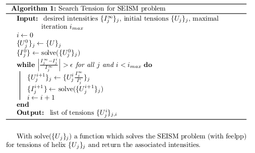
Algorithme of search of Tensions

We can represent this algorithm by diagram :

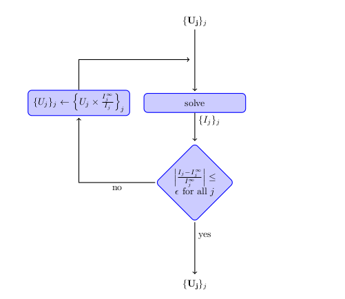
Diagram of search of Tensions

The solve function solves the static case to reduce the time of compute. The feelpp’s file of static simulation are here : seism_static.cfg and seism_static.json.

This algorithm is implement on python3’s language with feelpp the python’s module for feelpp : Edit the file.

11. Numeric Parameters

This section show the parameters used to compute the simulation.

Size of mesh :
- Near of Helix : \(h = 1 \, mm\)
- Near of Infinie : \(h = 10 \, mm\)
Time Parameters :
- Time step : I use adaptative time step. Near of brutal changement of current, the time step is little, in other case, the time step is big. I put adaptative time step to have good precision near of changement (cut of current at \(t=22s\)) and to not explose the time of compute. The shell script feelpp_adaptative.sh implements that.
  
  \(\Delta_t = \left\{ \begin{matrix} 0.1s \, \text{for} \, 0s<t<0.9s \\ 0.008s \, \text{for} \, 0.9s<t<1.1s \\ 0.1s \, \text{for} \, 1.1s<t<19.9s \\ 0.008s \, \text{for} \, 19.9s<t<20.1s \\ 0.1 \, \text{for} \, 20.1s<t<22s \end{matrix} \right.\)
- Initial Time : \(0 \, s\)
- Final Time : \(22 \, s\)
Element type : \(P2\) for magnetic equation (\(\mathbf{A}\) and \(P1\) heat equation (\(T\))

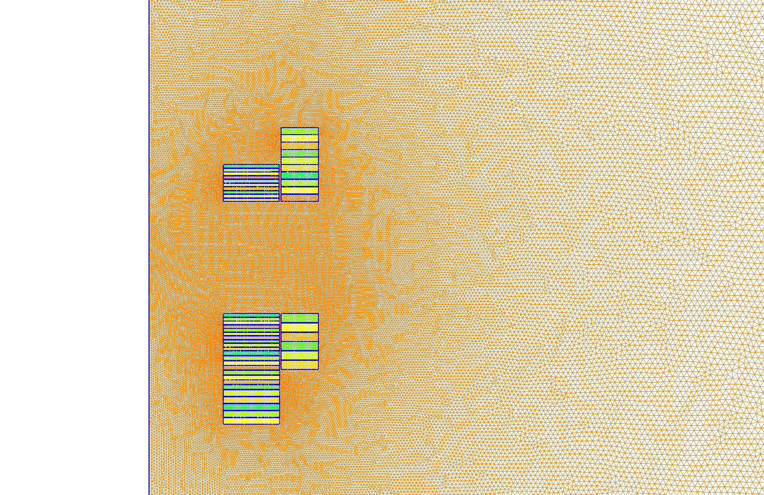
Mesh of Geometry

12. Results

12.1. Tensions

We obtain the tensions associate to intensities :

Physical Quantity

Helix1

Helix2

Helix3

Helix4

Helix5

Helix6

Unit

\(I\)

\(7000\)

\(-7000\)

\(7000\)

\(-7000\)

\(A\)

\(U\) for Linear case

\(-0.499\)

\(-0.734\)

\(-0.979\)

\(0.870\)

\(-0.828\)

\(0.929\)

\(Volt\)

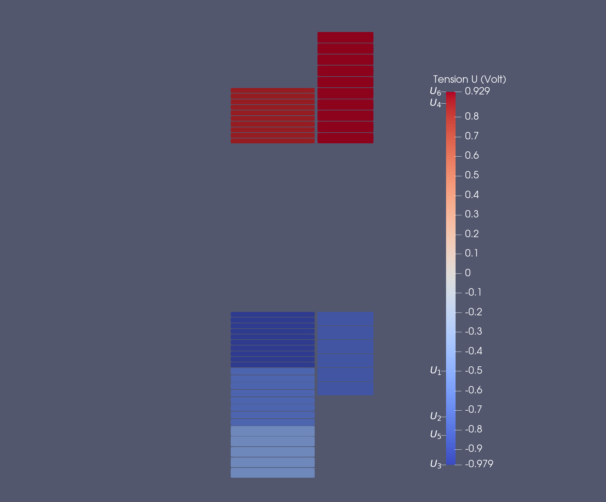
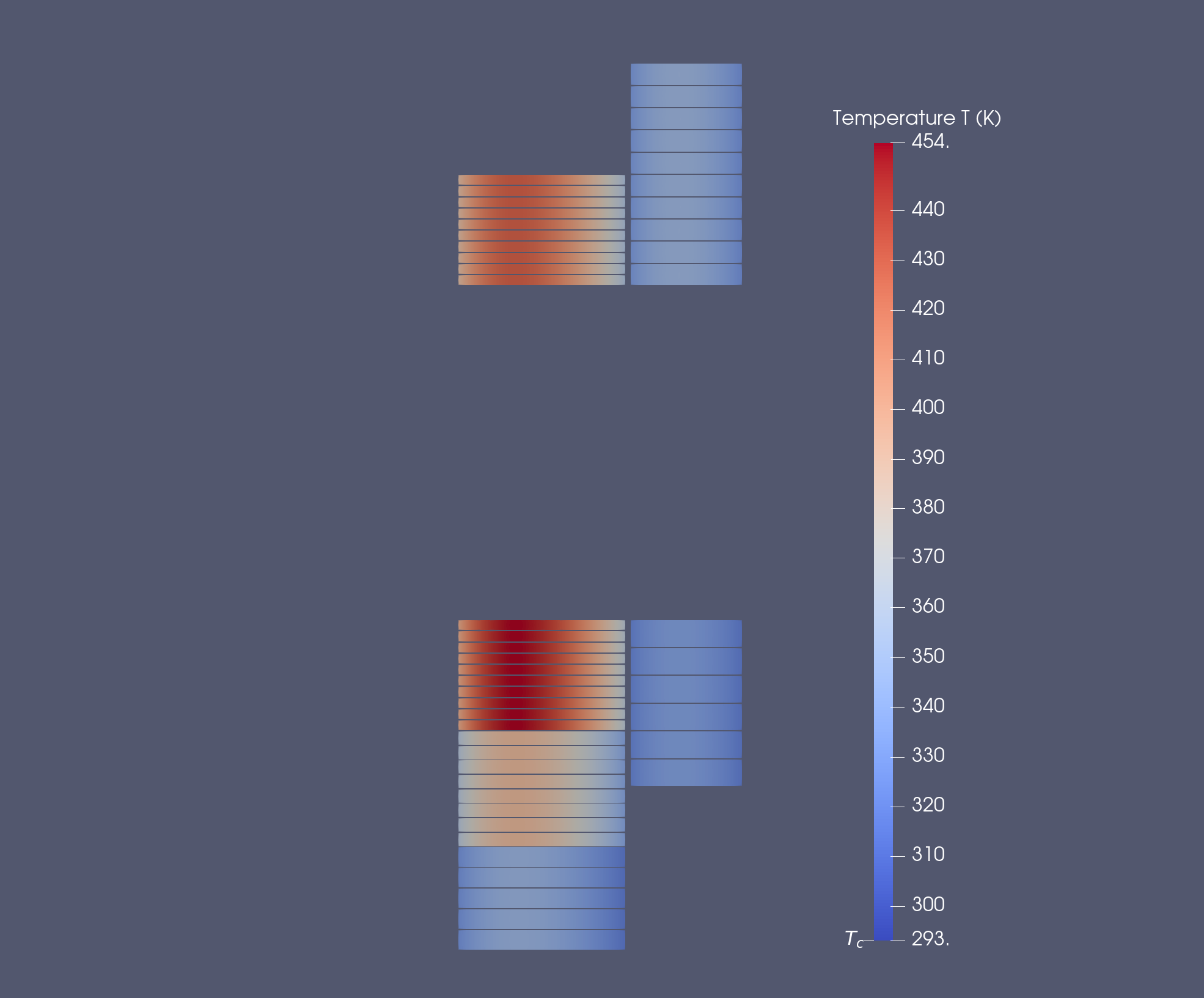
Tensions \(U (Volt)\) for Linear Case

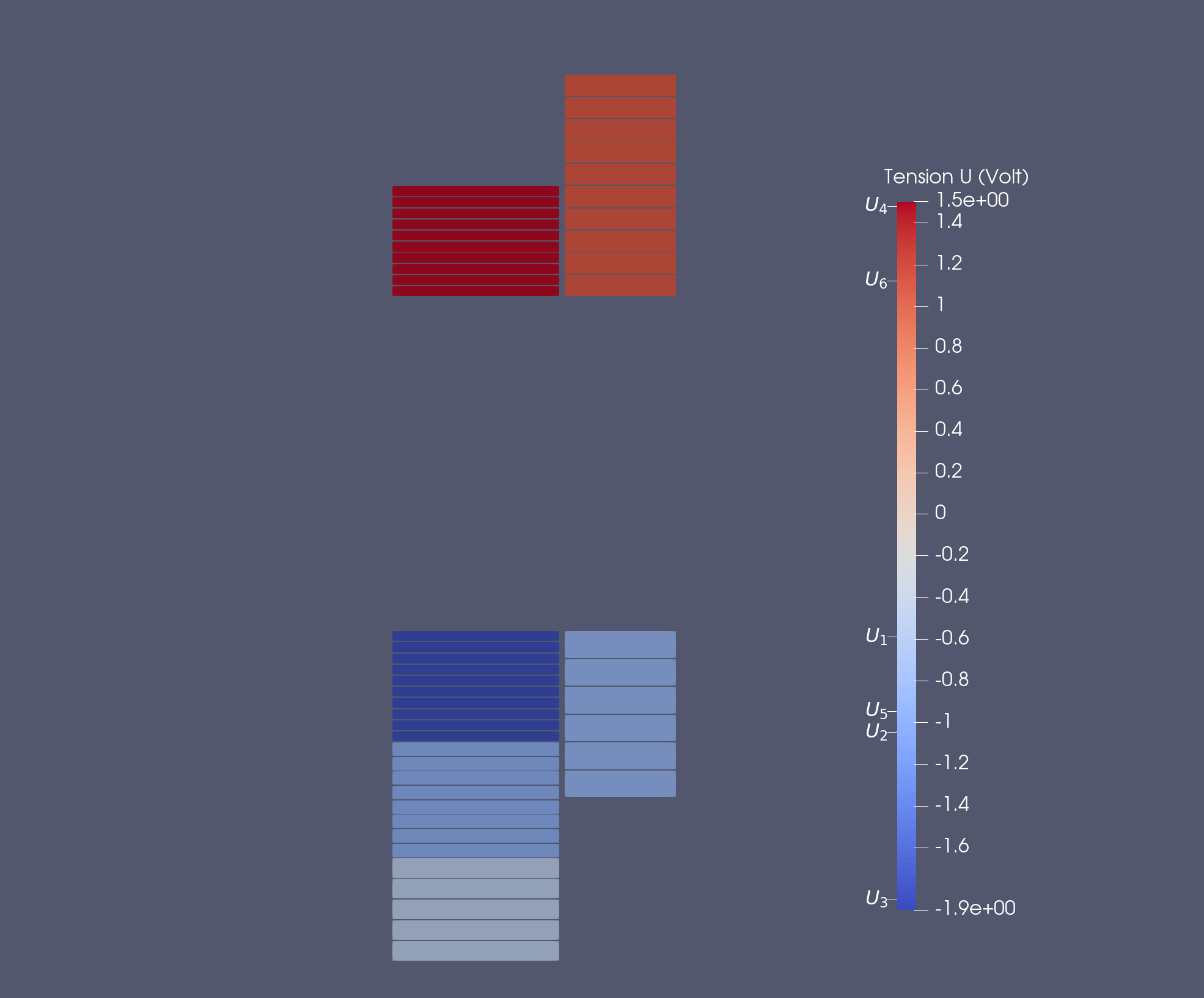
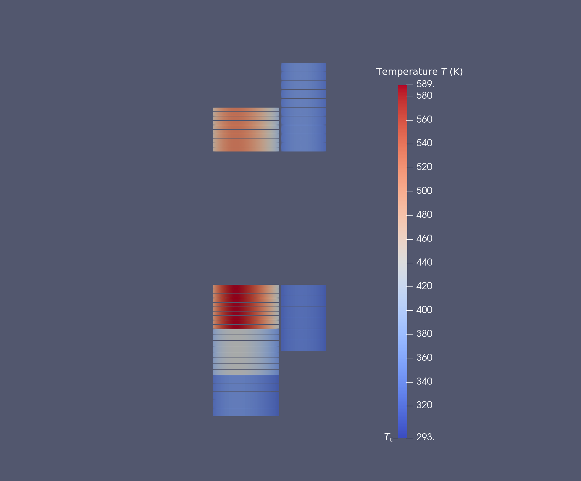
Tensions \(U (Volt)\) for Non-Linear Case

The algorithm of tension’s searching need 2 cycles for Linear case and 13 cycles for Non-Linear case to converge with the input relative error \(\epsilon = 1e-3\).

In fact, the algorithm guarantees an relative error on intensities of \(1e-14\) for Linear case. Is it normal because, we have \(U = R I\) with \(R\) a constant, thus :

We have : \(U^1_j = U^0_j \frac{I^{\infty}_j}{I^0_j}\)

In the other hand : \(U^0_j = R I^0_j\) and \(U^1_j = R I^1_j\)

Thus : \(R I^{\infty}_j = R I^1_j\) and \(I^1_j = I^{\infty}_j\)

For Non-Linear case, the resistances depends of intensities, thus with the same reasonment, we have just \(I^{i+1}_j = \frac{R^i_j}{R^{i+1}_j} \, I^{\infty}_j\).

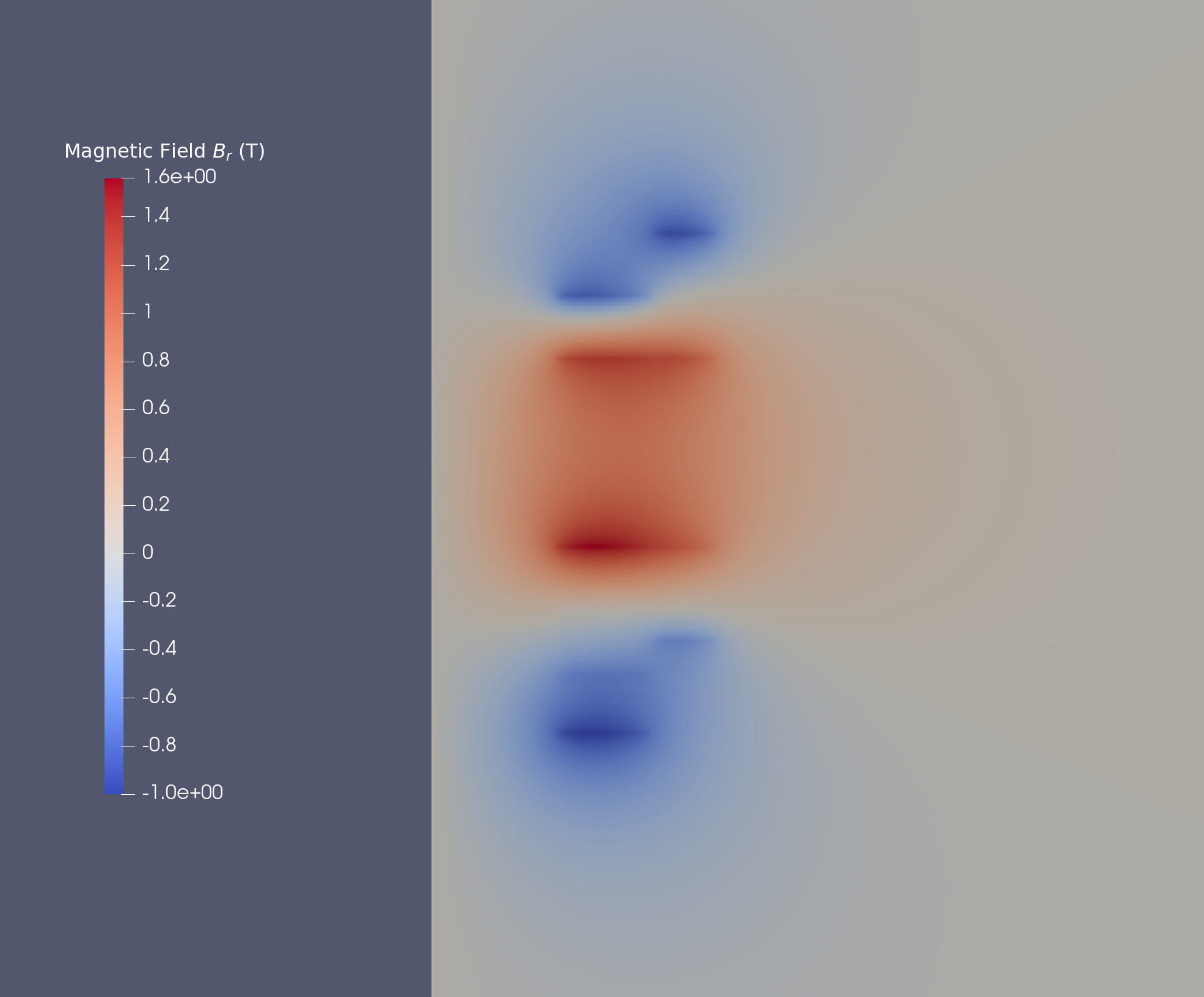
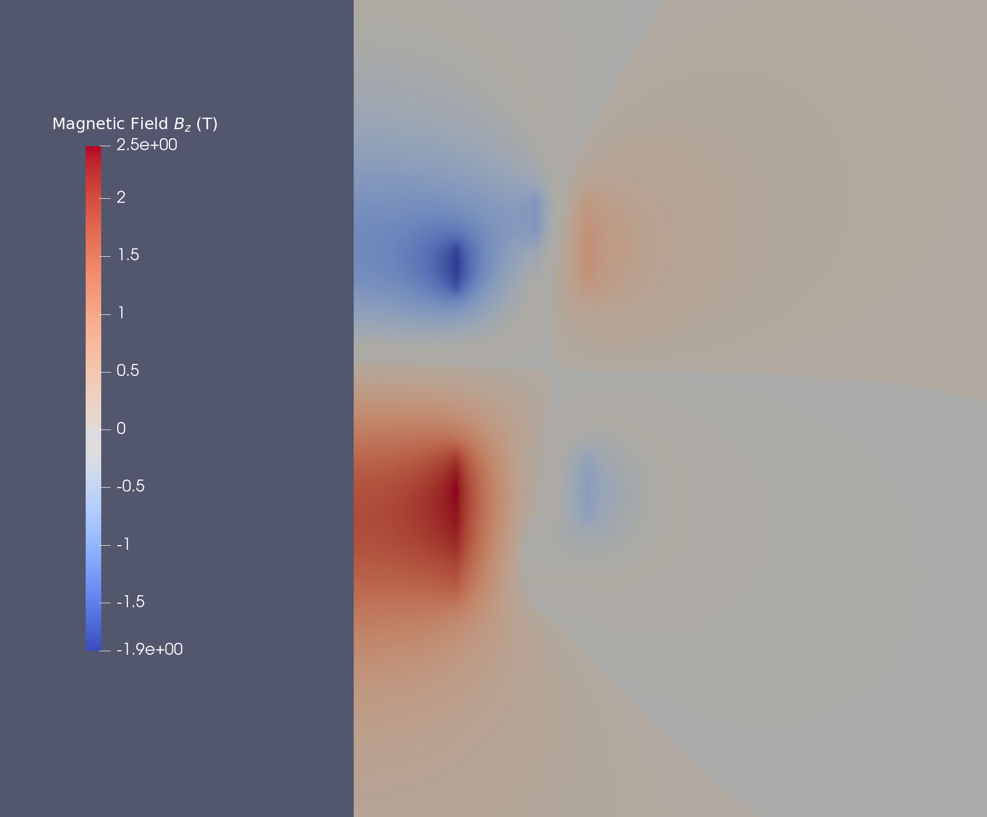
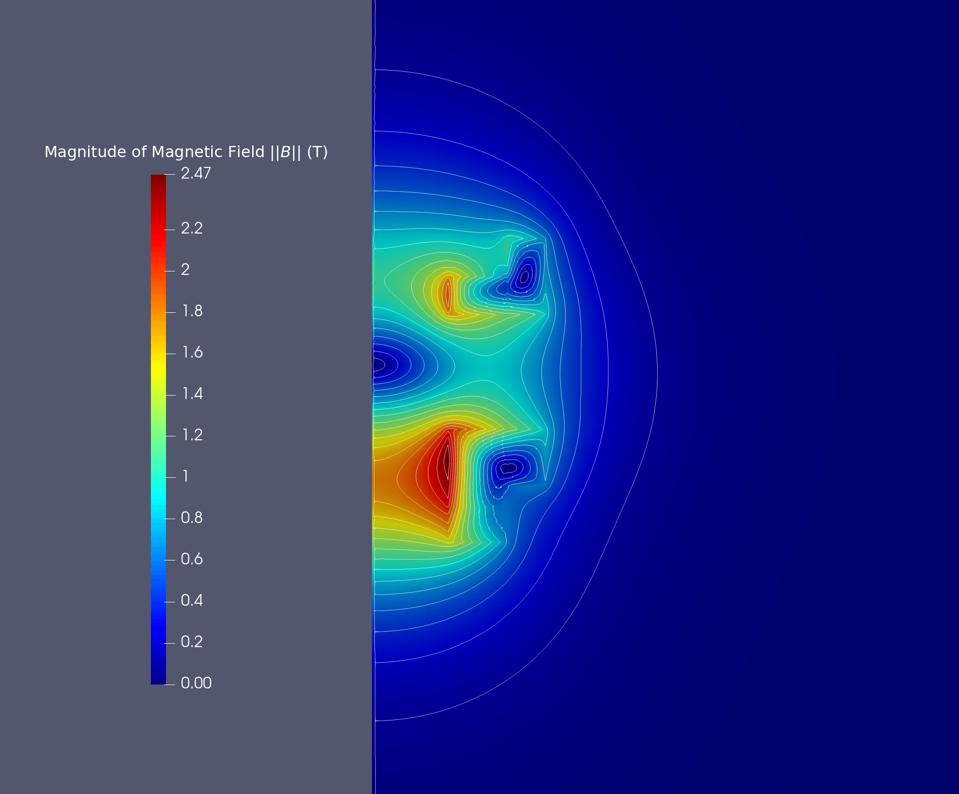
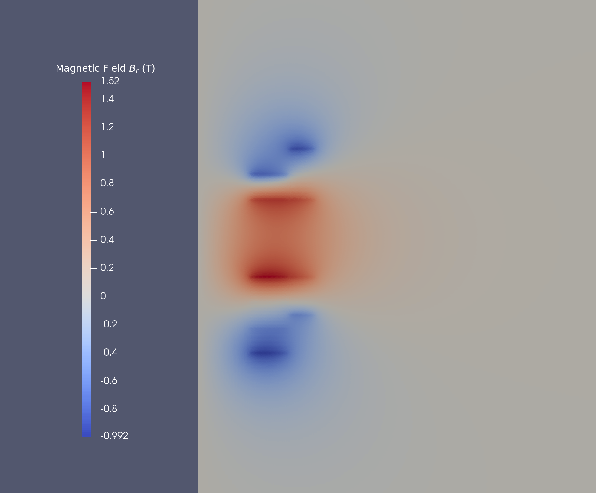
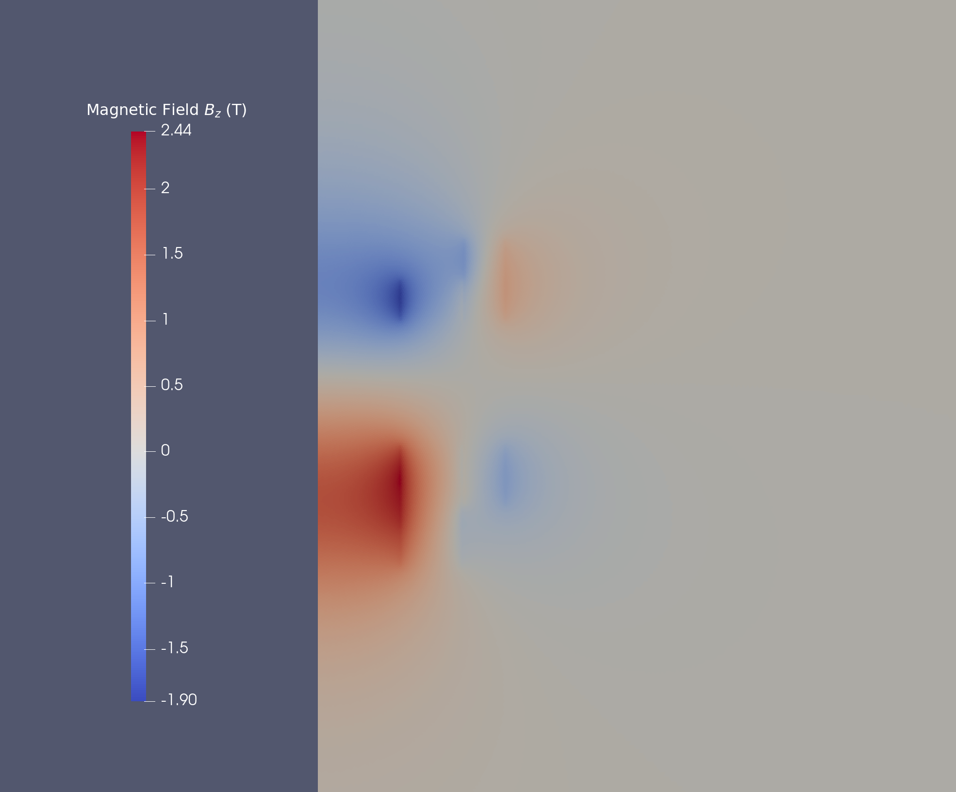
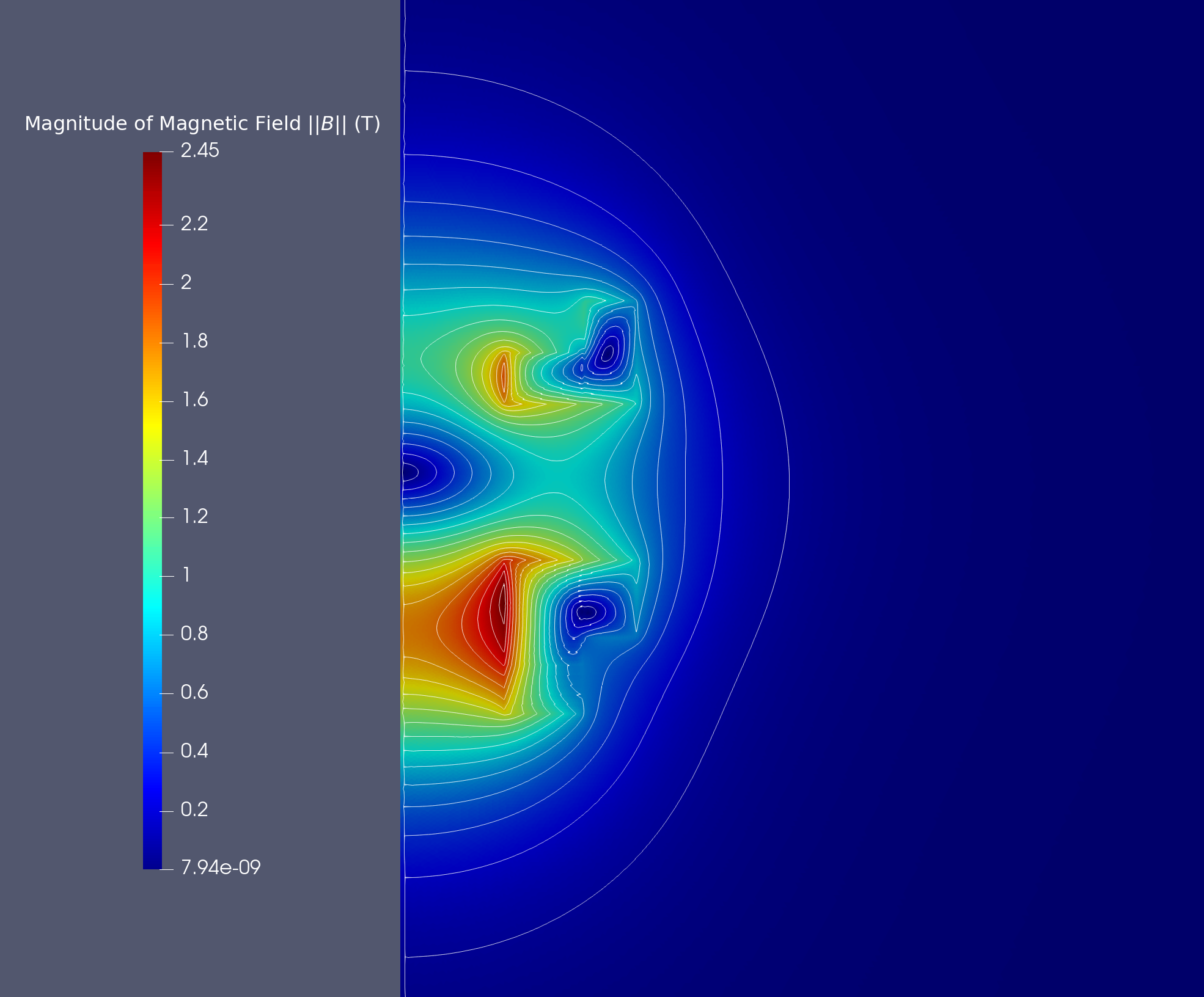
12.2. Magnetic Field

We obtain the magnetic field in stationnary case :

12.2.1. For Linear Case :

Radial Magnetic Field \(B_r (T)\)

Horizontal Magnetic Field \(B_z (T)\)

We can plot the level lines :

Level line of Magnitude of Magnetic Field \(\Vert B \Vert (T)\)

We can see in the center of magnets, the isobar lines form close shape, it is the ECR zone of SEISM.

12.2.2. For Non-Linear Case :

Radial Magnetic Field \(B_r (T)\)

Horizontal Magnetic Field \(B_z (T)\)

We can plot the level lines :

Level line of Magnitude of Magnetic Field \(\Vert B \Vert (T)\)

We can see in the center of magnets, the isobar lines form close shape, it is the ECR zone of SEISM.

12.3. Temperature

We obtain the temperature in stationnary case :

Temperature \(T (K)\) for Linear case

Temperature \(T (K)\) for Non-Linear case

The Non-Linear case searches a higher temperature than the Linear case : \(T_{max \, Non-Linear} = 569 \, K\) and \(T_{max \, Linear} = 454 \, K\).

13. Reference

Status of SEISM Experiments, M. Marie-Jeanne, J. Angot, P. Balint, November 29 2011, Sydney Australia Download the PDF

Laboratoire de Physique Subatomique & Cosmologie, IN2P3 (CNRS), Université Grenoble Alpes, website, link of website