Test case : One Torus

1. Introduction

In this page, I present the test case of Maxwell Quasi Static Problem in A-V Formulation with gauge condition for a geometry of torus surrounded by air for instationnary case in Axisymmetrical case.

2. Run the calculation

The command line to run this case is :

    mpirun -np 16 feelpp_toolbox_coefficientformpdes --config-file=mqs.cfg --cfpdes.gmsh.hsize=1e-3

3. Data Files

The case data files are available in Github here :

CFG file - Edit the file
JSON file - Edit the file
GEO file - Edit the file

4. Equation

We solve the A-V Formulation in axisymmetric and we assume that $V$ is known.

The unknow of equation is $\Phi = r \, A_{\theta}$ but we want Magnetic Potential field $A_{\theta}$ .

Differential Formulation

(AV Axis) ⎧ ⎪ ⎪ ⎪ ⎪ ⎪ ⎪ ⎪ ⎨ ⎪ ⎪ ⎪ ⎪ ⎪ ⎪ ⎪ ⎩ \begin{matrix} σ \frac{\partial Φ}{\partial t} - \frac{1}{μ} Δ Φ + \frac{2}{μ r} \frac{\partial Φ}{\partial r} + σ \frac{\partial V}{\partial θ} = 0 & on Ω^{a x i s} & (AV-1 Axis) V = \frac{U}{2 π} θ & on Ω_{c}^{a x i s} & (AV-2 Axis) A_{θ} = 0 & on Γ_{D}^{a x i s} & (D Axis) \frac{\partial A_{θ}}{\partial n^{a x i s}} = 0 & on Γ_{N}^{a x i s} & (N Axis) \end{matrix}

$\text{(AV Axis)} \left\{ \begin{matrix} \sigma \frac{\partial \Phi}{\partial t} - \frac{1}{\mu} \Delta \Phi + \frac{2}{\mu \, r} \frac{\partial \Phi}{\partial r} + \sigma \frac{\partial V}{\partial \theta} = 0 & \text{ on } \Omega^{axis} & \text{(AV-1 Axis)} \\ V = \frac{U}{2\pi} \, \theta & \text{ on } \Omega_c^{axis} & \text{(AV-2 Axis)} \\ A_{\theta} = 0 & \text{ on } \Gamma_D^{axis} & \text{(D Axis)} \\ \frac{\partial A_{\theta}}{\partial \mathbf{n}^{axis}} = 0 & \text{ on } \Gamma_N^{axis} & \text{(N Axis)} \end{matrix} \right.$

With :

$\Phi = r A_{\theta}$ : $A_{\theta}$ component $\theta$ of potential magnetic field
$\sigma$ : electric conductivity $S/m$
$\mu$ : electric permeability $kg/A^2/S^2$
$U$ : tension $Volt$

5. Geometry

The geometry is a torus of conductor in cartesian coordinates $(x,y,z)$ or rectangle in axisymmetric coordinates $(r,z)$ , surrounded by air.

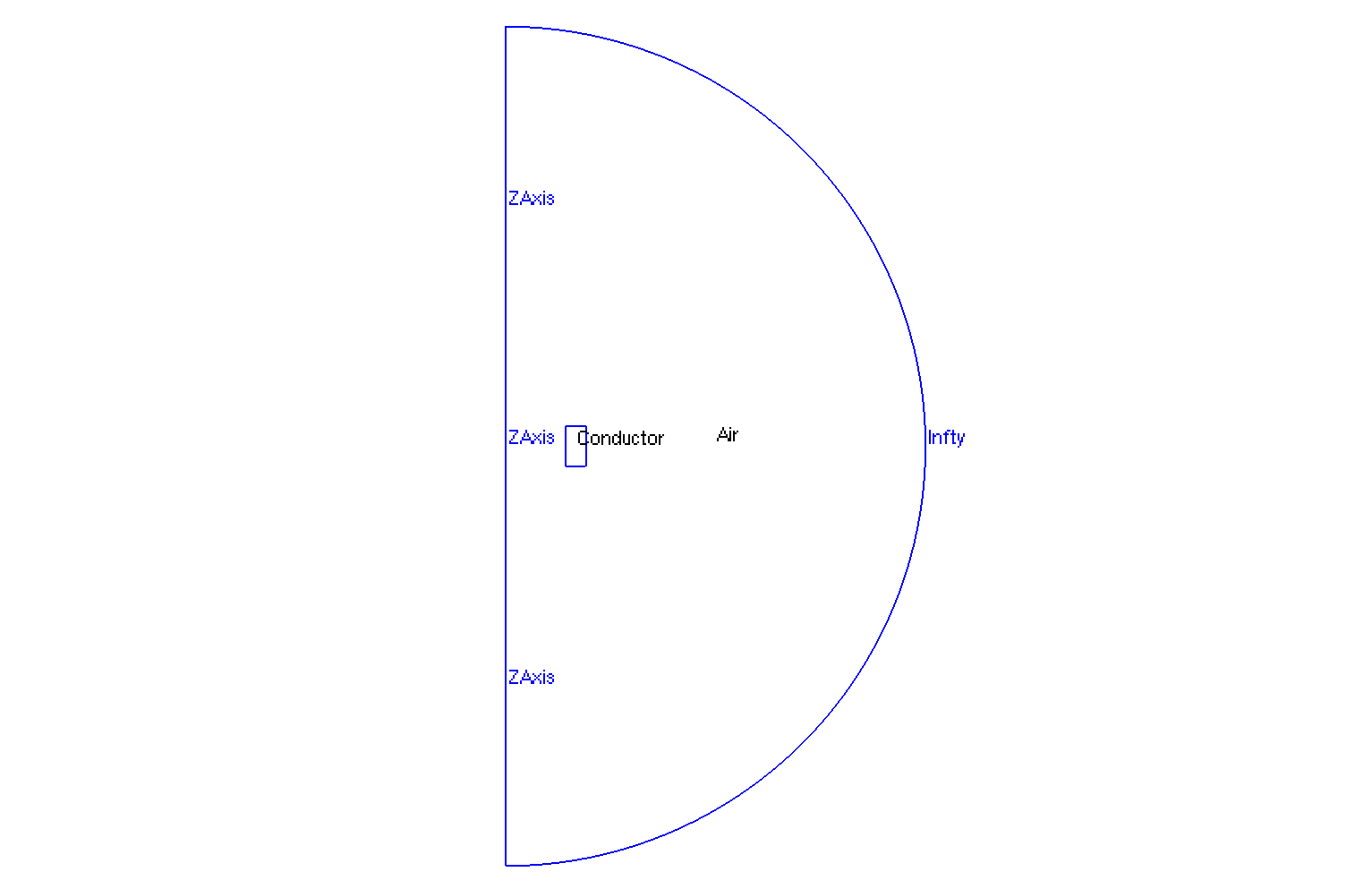
Geometry in Axisymmetrical cut

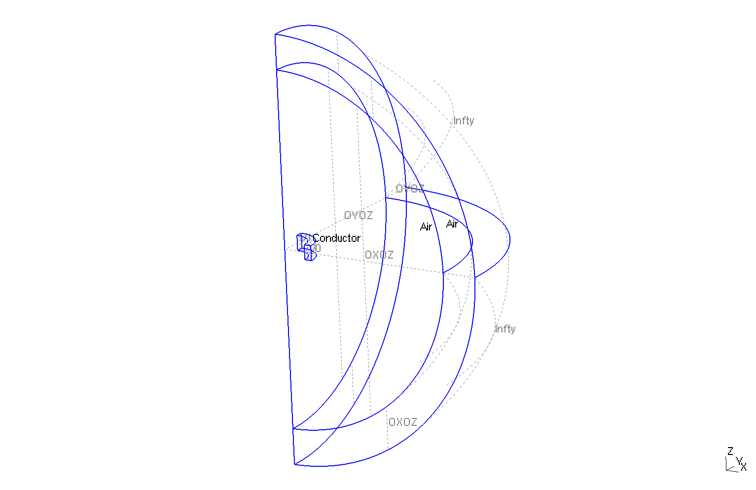
Geometry in three dimensions

The geometrical domains are :

Conductor : the torus, it is composed of conductive materials
Air : the air surround Conductor
- zAxis : a bound of Air, correspond to $zO$ axis ( $\{(z,r), \, z=0 \}$ )
- infty : the rest of bound of Air

Symbol

Description

value

unit

$r_{int}$

interior radius of torus

$75e-3$

$r_{ext}$

exterior radius of torus

$100.2e-3$

$z_1$

half-height of torus

$25e-3$

$r_{infty}$

radius of infty border

$5*r_{ext}$

6. Initial/Boundary Conditions

We impose the Dirichlet boundary conditions :

On zAxis : $\Phi = 0$ ( $A_{\theta} = 0$ by symetric argument)
On infty : $\Phi = 0$ ( $A_{\theta} = 0$ we consider the bound of resolution like infty for magnetic field)

We initialize :

On Conductor : $\Phi(t=0,r,z) = 0$ ( $A_{\theta}(t=0,r,z) = 0$ )
On Air : $\Phi(t=0,r,z) = 0$ ( $A_{\theta}(t=0,r,z) = 0$ )

On JSON file, the boundary conditions are writed :

Boundary conditions on JSON file

    "BoundaryConditions":
    {
        "magnetic":
        {
            "Dirichlet":
            {
                "ZAxis":
                {
                    "expr":"0"
                },
                "Infty":
                {
                    "expr":"0"
                }
            }
        }
    }

For initial condition, we write nothing in JSON, by default the application put zeros on initialization.

7. Weak Formulation

We obtain :

Weak Formulation

\int_{Ω^{a x i s}} σ \frac{\partial Φ}{\partial t} ϕ r d r d z + \int_{Ω^{a x i s}} \frac{1}{μ} ~ \nabla Φ \cdot ~ \nabla ϕ r d r d z + \int_{Ω^{a x i s}} \frac{2}{μ r} \frac{\partial Φ}{\partial r} ϕ r d r d z = - \int_{Ω_{c}^{a x i s}} σ \frac{\partial V}{\partial θ} ϕ r d r d z

$\scriptsize{ \int_{\Omega^{axis}}{ \sigma \frac{\partial \Phi}{\partial t} \phi \ r\ drdz} + \int_{\Omega^{axis}}{ \frac{1}{\mu} \tilde{\nabla} \Phi \cdot \tilde{\nabla} \phi \ r \ drdz } + \int_{\Omega^{axis}}{\frac{2}{\mu \, r} \frac{\partial \Phi}{\partial r} \, \phi \ r \ drdz} = - \int_{\Omega_c^{axis}}{ \sigma \frac{\partial V}{\partial \theta} \phi \ r \ drdz } }$

With $\tilde{\nabla} = \begin{pmatrix} \frac{\partial}{\partial r} \\ \frac{\partial}{\partial z} \end{pmatrix}$

8. Parameters

The parameters of problem are :

On Conductor :

Symbol

Description

Value

Unit

$V$

scalar electrical potential

$U \, \frac{\theta}{2\pi}$

$Volt$

$U$

electrical potential

$1$

$Volt / rad$

$\sigma$

electrical conductivity

$58e6$

$S/m$

$\mu=\mu_0$

magnetic permeability of vacuum

$4\pi.10^{-7}$

$kg \, m / A^2 / S^2$

On Air :

Symbol

Description

Value

Unit

$\mu=\mu_0$

magnetic permeability of vacuum

$4\pi.10^{-7}$

$kg \, m / A^2 / S^2$

On JSON file, the parameters are writed :

Parameters on JSON file

    "Parameters":
    {
	    "U":"t/(0.1*10)*(t<0.1*10)+(t<0.5*40)*(t>(0.1*10)):t" // Volt
    }

9. Coefficient Form PDEs

We use the application Coefficient Form PDEs. The coefficient associate to Weak Formulation are :

On Conductor :

Coefficient

Description

Expression

$d$

damping or mass coefficient

$\sigma$

$c$

diffusion coefficient

$\frac{r}{\mu}$

$\beta$

convection coefficient

$\begin{pmatrix} \frac{2}{\mu} \\ 0 \end{pmatrix}$

$f$

source term

$- \sigma \frac{U}{2\pi} \, r$

On Air :

Coefficient

Description

Expression

$c$

diffusion coefficient

$\frac{r}{\mu}$

$\beta$

convection coefficient

$\begin{pmatrix} \frac{2}{\mu} \\ 0 \end{pmatrix}$

On JSON file, the coefficients are writed :

CFPDEs coefficients on JSON file

    "Materials":
    {
        "Conductor":
        {
            "sigma":58e+6,      // S.m-1
            "mu":"4*pi*1e-7",   // kg.m/A2/S2
	        "magnetic_c":"x/mu:x:mu",
            "magnetic_beta":"{2/mu,0}:mu",
            "magnetic_f":"-sigma*U/2/pi*x:sigma:U:x:mu",
            "magnetic_d":"sigma*x:x:sigma"
        },
        "Air":
        {
            "mu":"4*pi*1e-7",   // kg.m/A2/s2
            "magnetic_c":"x/mu:x:mu",
            "magnetic_beta":"{2/mu,0}:mu"
        }
    }

10. Numeric Parameters

Time
- Initial Time : $0s$
- Final Time : $240s$
- Time Step : $10s$
Mesh size :
- Interior of torus : $0.001 m$
- Far of torus : $0.004 m$

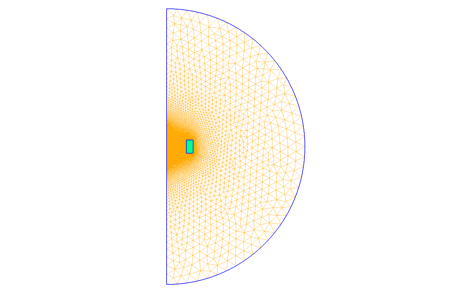
Mesh of Geometry

11. Export

We solve an equation (A-V Formulation in axisymmetric) of unknow $\Phi = r \, A_{\theta}$ but we want the magnetic field $\mathbf{B}$ .

The potential magntic vector $\mathbf{A}$ is define :

$\mathbf{B} = \nabla \times \mathbf{A}$

So, with rotational in cylindric and axisymmetric condition :

$\mathbf{B} = \begin{pmatrix} B_r \\ B_{\theta} \\ B_z \end{pmatrix} = \begin{pmatrix} - \frac{\partial A_{\theta}}{\partial z} \\ 0 \\ \frac{1}{r} \frac{\partial \left( r A_{\theta} \right)}{\partial r} \end{pmatrix}$

We export from $\Phi$ :

$A_{\theta} = \frac{\Phi}{r}$
$B_r = - \frac{1}{r} \frac{\partial \Phi}{\partial z}$
$B_z = \frac{1}{r} \frac{\partial \Phi}{\partial r}$

12. Run the calculation

12.1. CFPDEs

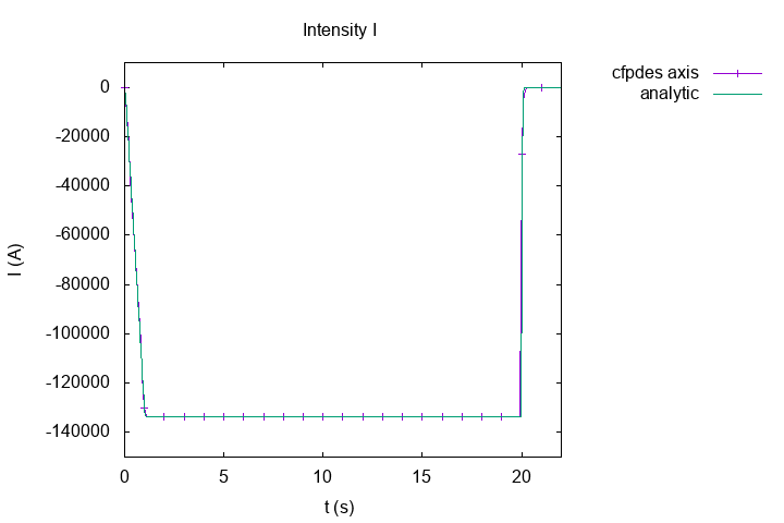
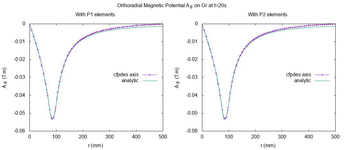
13. Result

The analytical solve of potential magnetic field and magnetic field (the cyan curve on plots) is computed by python3’s module MagnetTools.MagnetTools. The module based on paper : spire.

The analytical solve of intensity (and magnetic field) is computed on python3’s script Edit the file.

13.1. Intensity

I plot the intensity of current with analytical solve.

Intensity

$I (A)$

13.2. Magnetic Potential Field

Orthoraidal Magnetic Potential Field

$A_{\theta} (T.m)$

13.2.1. On Or axis at $t=20s$

I export the magnetic potential field at $t=20s$ because we consider at this time, the system is stationary. Thus, we can compare with the analytical solve of stationnary problem.

$A_{\theta} (A/m^2)$ on Or axis

13.3. Magnetic Field

Horizontal Magnetic Field

$B_z (T)$

13.3.1. On Or axis at $t=20s$

I export the magnetic field at $t=20s$ because we consider at this time, the system is stationary. Thus, we can compare with the analytical solve of stationnary problem.

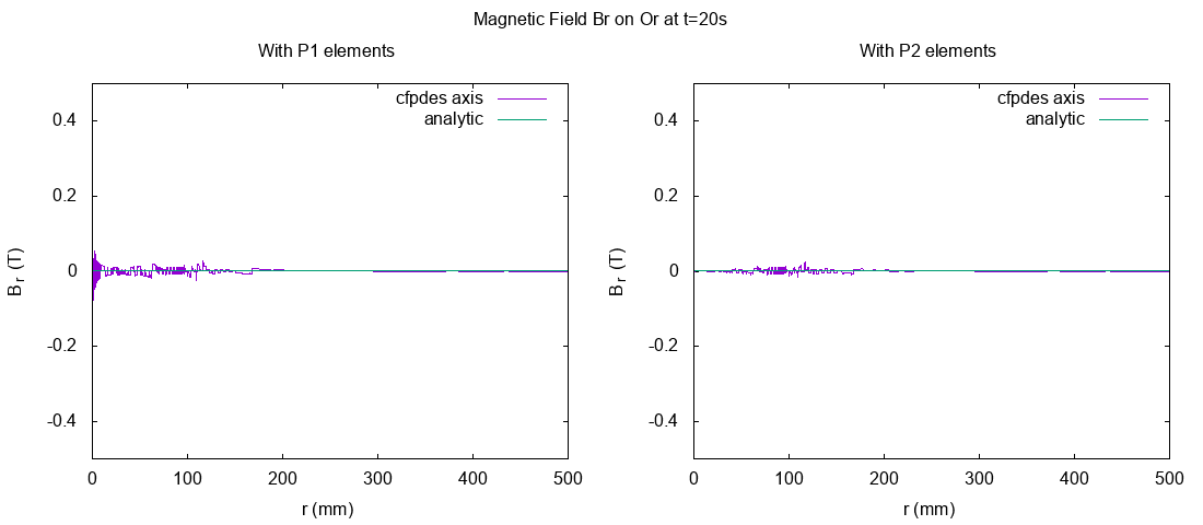
$B_r (T)$ on Or axis

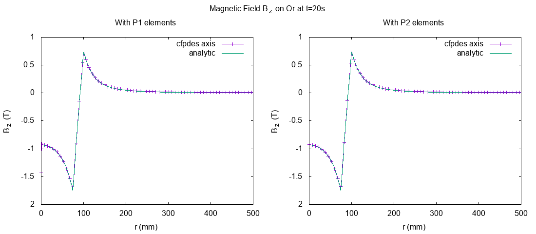
$B_z (T)$ on Or axis

Around the Or axis, the direction of Magnetic field $B$ is horizontal, in particulary at $P0=(r=0,z=0)$ .

We can observe a great difference between the resolution with P1 and P2 elements at $r=0$ :

$B_z (T)$ on Or axis

The result in P1 elements have instability near of $r=0$ but not with $P2$ . This instability can be explain by the method of export of Magnetic Field : to have $B_z$ , we export $\frac{1}{r} \frac{\partial \Phi}{\partial r}$ and the division $\frac{1}{r}$ near of $r=0$ can be a problem.

13.3.2. On $P0=(r=0,z=0)$ in terms of time

The value of magnetic field on $P0=(r=0,z=0)$ is important because the research put theire experiments near of this point.

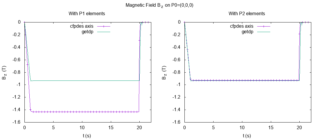
$B_z (T)$ on P0

We can see a difference between the result $B_z$ with P1 and P2 element. The curve of z-magnetic field $B_z$ in P1 element is far of analytical solve and in P2, it seems good. The phenomena is explain by the remark above.

14. References

Calcul du champ magnétique pour les géométries axisymétriques simples, Christophe Trophime, 2002, unpublished, Download the PDF

Test case : One Torus

1. Introduction

2. Run the calculation

3. Data Files

4. Equation

5. Geometry

6. Initial/Boundary Conditions

7. Weak Formulation

8. Parameters

9. Coefficient Form PDEs

10. Numeric Parameters

11. Export

12. Run the calculation

12.1. CFPDEs

13. Result

13.1. Intensity

13.2. Magnetic Potential Field

13.2.1. On Or axis at t=20st=20s

13.3. Magnetic Field

13.3.1. On Or axis at t=20st=20s

13.3.2. On P0=(r=0,z=0)P0=(r=0,z=0) in terms of time

14. References

13.2.1. On Or axis at $t=20s$

13.3.1. On Or axis at $t=20s$

13.3.2. On $P0=(r=0,z=0)$ in terms of time