Elastic Equations with Electromagnetism and Thermic

In page Equations of Elasticity in Static case and Equations of Elasticity in Transient case, we show the elastic equations on axisymmetrical geometry and a method of ximeric solve with CFPDEs.

Now, in this section, we want two coupled those elasticity equations with AV-Formulation and Heat Equation in transient and static case.

The electromagnetism have a contribution in deformation of geometry by Laplace Force. The thermic have a contribution in deformation of geometry by Thermal Dilatation.

diagram physics
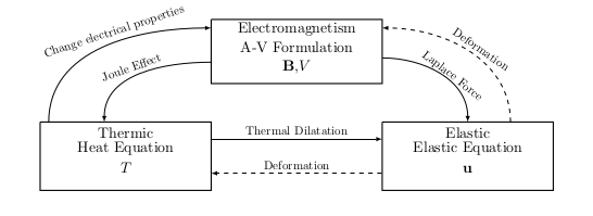
Diagram of Coupling problem

1. Recall

1.1. Electromagnetism

This section recall the content of page A-V Formulation.

The electromagnetism is one of four elementary force. It is the origin of many phenomena. The LNCMI search to reach highest magnetism field with its magnets.

A electromagnetism system is describe by electric field \(\mathbf{E}\) and magnetism field \(\mathbf{B}\). This two values are governed by Maxwell Equation. We place on Maxwell Quasi Static Case :

Maxwell Equations in MQS
\[\begin{align*} \nabla \times \textbf{H}(\textbf{x}, t) &= \textbf{J}(\textbf{x}, t) & \text{ (Maxwell-Ampere)}\\ \nabla \times \textbf{E}(\textbf{x}, t) &= - \frac{\partial \textbf{B}}{\partial t}(\textbf{x}, t) & \text{ (Maxwell-Faraday)} \\ \nabla \cdot \textbf{B}(\textbf{x}, t) &= 0 & \text{ (Maxwell-Thomson)} \\ \mathbf{J}(\mathbf{x},t) &= \sigma \, \mathbf{E}(\mathbf{x},t) \\ \textbf{B}(\textbf{x}, t) &= \mu \, \textbf{H}(\textbf{x}, t) \end{align*}\]

With :

  • \(\textbf{H}(\textbf{x},t)\) magnetic field intensity (\(A m^{-1}\))

  • \(\textbf{E}(\textbf{x},t)\) electric field intensity (\(V m^{-1}\))

  • \(\textbf{B}(\textbf{x},t)\) magnetic induction density (\(T\))

  • \(\textbf{J}(\textbf{x},t)\) current density (\(A m^{-2}\))

  • \(\mu(\textbf{x},t)\) permeability (\(H m^{-1}\))

  • \(\sigma(\textbf{x},t)\) conductivity (\(S m^{-1}\))

With those equations, we add the conservation of current density :

\[ \nabla \cdot \mathbf{J} = 0\]

We can introduce the magnetic potential field \(\mathbf{A}\) :

\[ \mathbf{B} = \nabla \times \mathbf{A}\]

With gauge condition :

\[ \nabla \cdot \mathbf{A} = 0\]

And electric potential scalar \(V\) :

\[ \nabla V = - \mathbf{E} - \frac{d \mathbf{A}}{d t}\]

With those new values, we can rewrite the Maxwell Equations in MQS in A-V Formulation with Dirichlet and Neumann conditions :

A-V Formulation
\[\text{(AV Formulation)} \left\{ \begin{matrix} \nabla \times \left( \frac{1}{\mu} \nabla \times \textbf{A} \right) + \sigma \frac{\partial \textbf{A}}{\partial t} + \sigma \nabla V &=& 0 \text{ on } \Omega & \text{(AV-1)} \\ \nabla \cdot \left( \sigma \nabla V + \sigma \frac{\partial \textbf{A}}{\partial t} \right) &=& 0 \text{ on } \Omega_c & \text{(AV-2)} \\ \mathbf{A} \times \mathbf{n} &=& 0 \text{ on } \Gamma_D & \text{(AV-D)} \\ \left( \nabla \times \mathbf{A} \right) \times \mathbf{n} &=& 0 \text{ on } \Gamma_N & \text{(AV-N)} \end{matrix} \right.\]

1.2. Thermic

The temperature is the physic phenomena of micro movements of atoms. When a current pass in electrical ressistive matters, those matters emits heat and increase its temperature. Thise temperature can reduce the performance of magnet and, worst, contribute to broke it. This contraint must be modelize to understand the phenomena in magnet.

The themperature is governed by Heat Equation :

Heat Equation
\[\text{(Heat)} \left\{ \begin{matrix} \rho C_p \, \frac{\partial T}{\partial t} - k \Delta T = Q & \text{ on } \Omega_c & \text{(Heat-1)} \\ \frac{\partial T}{\partial \mathbf{n}} = 0 & \text{ on } \Gamma_{Nc} & \text{(Heat-N)} \\ - k \, \frac{\partial T}{\partial \mathbf{n}} = h \, \left( T - T_c \right) & \text{ on } \Gamma_{Rc} & \text{(Heat-R)} \\ \end{matrix} \right.\]

With :

  • \(T\) : temperature \((K)\)

  • \(\rho\) : density \((kg/m^3)\)

  • \(C_p\) : thermal capacity \((J/K/kg)\)

  • \(k\) : thermal conductivity \((W/m/K)\)

  • \(Q\) : source term \((K)\)

  • \(h\) : convection coefficient \((W \, m^{-2} / K)\)

The magnet is cooling by water in high pressure, it’s represented by Robin’s conditions : \(- k \, \frac{\partial T}{\partial \mathbf{n}} = h \, \left( T - T_c \right)\) with \(T_c\) the temperature of cooling and \(h\) the convertion coefficient between the magnet matters of magnet (here a copper) and the water.

As we said before, the magnet emits heat when a current pass. This phenomena is represented by source term \(Q\) which depends of current density \(\mathbf{J}\) and magnetic field \(\mathbf{B}\) :

\[ Q = \mathbf{J} \cdot \mathbf{B}\]

With potentials :

\[ Q = \sigma \left( \nabla V + \frac{d \mathbf{A}}{d t} \right) \cdot \left( \nabla V + \frac{d \mathbf{A}}{d t} \right)\]

1.3. Materials properties

Certain parameters of matters changed in function of temperature. For metals we have :

  • Electrical conductivity :

    \[ \sigma(T) = \frac{\sigma_0}{1 + \alpha (T-T_0)}\]

    with : reference temperature \(T_0\), reference conductivity \(\sigma_0=\sigma(T_0)\) and coeffcient \(\alpha\)

  • Thermal conductivity :

    \[ k(T) = \frac{k_0}{1 + \alpha (T-T_0)} \, \frac{T}{T_0}\]

    with : reference temperature \(T_0\), reference conductivity \(k_0=k(T_0)\) and coeffcient \(\alpha\)

With Ohm law : \(\mathbf{J} = \sigma(T) \mathbf{E}\), the higher the temperature, the higher the resistance and the lower the current flow.

1.4. Thermo-magnetism model

We have the thermo-magnetism model :

Differential Formulation
\[\small{ \left\{ \begin{matrix} \nabla \times \left( \frac{1}{\mu} \nabla \times \textbf{A} \right) + \sigma(T) \frac{\partial \textbf{A}}{\partial t} + \sigma(T) \nabla V &=& 0 & \text{ on } \Omega & \text{(AV-1)} \\ \nabla \cdot \left( \sigma(T) \nabla V + \sigma(T) \frac{\partial \textbf{A}}{\partial t} \right) &=& 0 & \text{ on } \Omega_c & \text{(AV-2)} \\ \rho C_p \, \frac{\partial T}{\partial t} - k(T) \Delta T &=& \sigma(T) \left( \nabla V + \frac{\partial \mathbf{A}}{\partial t} \right) \cdot \left( \nabla V + \frac{\partial \mathbf{A}}{\partial t} \right) & \text{ on } \Omega_c & \text{(Heat-1)} \\ \mathbf{A} \times \mathbf{n} &=& 0 & \text{ on } \Gamma_D & \text{(AV-D)} \\ \left( \nabla \times \mathbf{A} \right) \times \mathbf{n} &=& 0 & \text{ on } \Gamma_N & \text{(AV-N)} \\ \frac{\partial T}{\partial \mathbf{n}} &=& 0 & \text{ on } \Gamma_{Nc} & \text{(Heat-N)} \\ - k(T) \, \frac{\partial T}{\partial \mathbf{n}} &=& h \, \left( T - T_c \right) & \text{ on } \Gamma_{Rc} & \text{(Heat-R)} \\ \end{matrix} \right. }\]

With :

  • \(\mathbf{A}\) magnetic potential field

  • \(T\) temperature

  • \(V\) electrical potential scalar

  • \(k(T)=\frac{k_0}{1+\alpha (T-T_0)} \frac{T}{T_0}\) thermal conductivity

  • \(\sigma(T)=\frac{\sigma_0}{1+\alpha (T-T_0)}\) electrical conductivity

  • \(\rho\) density

  • \(C_p\) thermal capacity

  • \(T_c\) cooling temperature

  • \(T_0\) reference temperature

1.5. Elastic Equation

The electromagnetism create solid contraints on magnet (it’s Laplace Force). To understand thise phenomena, we must to expose the elastic equations. They govern the deformation of matters.

We introduce :

  • The displacemant \(\mathbf{u} = \begin{pmatrix} u_x \\ u_y \\ u_z \end{pmatrix}\)

  • The tensor of small deformation : \(\bar{\bar{\epsilon}} = \frac{1}{2} \left( \nabla \mathbf{u} + \nabla \mathbf{u}^T \right)\)

  • The stress tensor : \(\bar{\bar{\sigma}} = C(\bar{\bar{\epsilon}})\) with \(C\) a tensor which depends of the choice of elastic law.

  • The volumic Force : \(\mathbf{F}\)

Differential Formulation of Elasticity Equation
\[\text{(Elasticity)} \\ \left\{ \begin{matrix} \frac{\partial \mathbf{p}}{\partial t} - \nabla \cdot \bar{\bar{\sigma}} = \mathbf{F} & \text{on } \Omega_c & \text{(Elas-1)} \\ \mathbf{u} = \mathbf{u_0} & \text{on } \Gamma_{D \hspace{0.05cm} elas} & \text{(Elas-D)} \\ \bar{\bar{\sigma}} \cdot \mathbf{n} = g_N & \text{on } \Gamma_{N \hspace{0.05cm} elas} & \text{(Elas-N)} \\ \bar{\bar{\sigma}} \cdot \mathbf{n} + k \, \mathbf{u} = g_R & \text{on } \Gamma_{R \hspace{0.05cm} elas} & \text{(Elas-R)} \end{matrix} \right.\]

With :

  • Lamé’s coefficients : \(\lambda = \frac{E \, v}{(1-2 v) \, (1+v)}\), \(\mu = \frac{E}{2 \, (1+v)}\) with

    • Young modulus \(E\)

    • Poisson’s coefficient \(v\)

  • Displacement \(\mathbf{u} = \begin{pmatrix} u_x \\ u_y \\ u_z \end{pmatrix}\)

  • Momentum \(\mathbf{p} = \frac{\partial \left( \rho \, \mathbf{u} \right)}{\partial t} = \begin{pmatrix} p_x \\ p_y \\ p_z \end{pmatrix}\) with \(\rho\) the density

  • Stress Tensor : \(\bar{\bar{\sigma}}\)

  • Stiffness tensor : \(k\)

  • Volumic Force : \(\mathbf{F}\)

And notations :

  • Divergence of tensor : \(\nabla \cdot \bar{\bar{\sigma}} = \begin{pmatrix} \nabla \cdot \bar{\bar{\sigma}}_{x,:} \\ \nabla \cdot \bar{\bar{\sigma}}_{y,:} \\ \nabla \cdot \bar{\bar{\sigma}}_{z,:} \end{pmatrix} = \begin{pmatrix} \frac{\partial \bar{\bar{\sigma}}_{xx}}{\partial x} + \frac{\partial \bar{\bar{\sigma}}_{xy}}{\partial y} + \frac{\partial \bar{\bar{\sigma}}_{xz}}{\partial z} \\ \frac{\partial \bar{\bar{\sigma}}_{yx}}{\partial x} + \frac{\partial \bar{\bar{\sigma}}_{yy}}{\partial y} + \frac{\partial \bar{\bar{\sigma}}_{yz}}{\partial z} \\ \frac{\partial \bar{\bar{\sigma}}_{zx}}{\partial x} + \frac{\partial \bar{\bar{\sigma}}_{zy}}{\partial y} + \frac{\partial \bar{\bar{\sigma}}_{zz}}{\partial z} \end{pmatrix}\)

  • Scalar produce of tensor : \(\bar{\bar{\sigma}} \cdot \mathbf{n} = \begin{pmatrix} \bar{\bar{\sigma}}_{x,:} \cdot \mathbf{n} \\ \bar{\bar{\sigma}}_{y,:} \cdot \mathbf{n} \\ \bar{\bar{\sigma}}_{z,:} \cdot \mathbf{n} \end{pmatrix} = \begin{pmatrix} \bar{\bar{\sigma}}_{xx} \, n_x + \bar{\bar{\sigma}}_{xy} \, n_y + \bar{\bar{\sigma}}_{xz} \, n_z \\ \bar{\bar{\sigma}}_{yx} \, n_x + \bar{\bar{\sigma}}_{yy} \, n_y + \bar{\bar{\sigma}}_{yz} \, n_z \\ \bar{\bar{\sigma}}_{zx} \, n_x + \bar{\bar{\sigma}}_{zy} \, n_y + \bar{\bar{\sigma}}_{zz} \, n_z \end{pmatrix}\)

The Hook’s law, it’s a law of linear elasticity (the basic model for linear matters) :

\[ \bar{\bar{\sigma}}^E = \lambda \, Tr(\bar{\bar{\epsilon}}) \, Id + 2\mu \, \bar{\bar{\epsilon}}\]

2. Laplace Force

The Laplace Force is the macroscopic result of Lorentz Force.

The circulation of current in conductor create movement of particle of charge. The Lorentz Force is the combination of electric and magnetic force. A particle of charge \(q\) moving with a velocity \(\mathbf{v}\) in an electric field \(\mathbf{E}\) and a magnetic field \(\mathbf{B}\) give :

\[ \mathbf{F}_{lorentz} = q \, \mathbf{E} + q \, \mathbf{v} \times \mathbf{B}\]

With Action-Reaction law, the stationary charges of conductor react to the Lorentz Force of moving charges. The result is a macroscopic force Laplace Force.

Thise force express with electric field \(\mathbf{E}\) and current density \(\mathbf{J}\) :

\[ \mathbf{F}_{laplace} = \mathbf{J} \times \mathbf{B}\]

With equation \(\mathbf{J}=\sigma \, \mathbf{E}\) definition of magnetic potential field \(\mathbf{A}\) and electric potential scalar \(V\), we can rewrite :

\[ \mathbf{F}_{laplace} = \left( \sigma \, \left( - \nabla V - \frac{d \mathbf{A}}{d t} \right) \right) \times \left( \nabla \times \mathbf{A} \right)\]

3. Thermal Dilatation

The temperature is the physic phenomena of micro movements of atoms of matters. The higher the temperature, the more the atoms take up space and the matter expands.

To modelize this thermal dilatation, we add a dilatation term to stress tensor of Hook’s law :

\[ \bar{\bar{\sigma}}(\bar{\bar{\epsilon}}) = \bar{\bar{\sigma}}^E(\bar{\bar{\epsilon}}) + \bar{\bar{\sigma}}^T(\bar{\bar{\epsilon}})\]

With :

  • term of Hook’s law : \(\bar{\bar{\sigma}}^E(\bar{\bar{\epsilon}}) = \lambda \, Tr(\bar{\bar{\epsilon}}) + 2\mu \bar{\bar{\epsilon}}\)

  • Dilatation term : \(\bar{\bar{\sigma}}^T(\bar{\bar{\epsilon}}) = - \left( 3\lambda + 2\mu \right) \, \alpha_T \, \left( T - T_0 \right) \, Id\), with linear dilatation coefficient \(\alpha_T\) and the reference temperature \(T_0\)

4. Elastic Thermic Electromagnetism model

4.1. Differential Equation

If we combine the Thermo-magnetism model and Elastic Equation with Lorents Force and Thermal Dilatation we obtain the equation :

Differential Formulation of Elastic Thermic Electromagnetism Equations
\[\small{ \text{(Elasto-Thermo-Elec)} \\ \left\{ \begin{align*} \nabla \times \left( \frac{1}{\mu} \nabla \times \textbf{A} \right) + \sigma(T) \frac{\partial \textbf{A}}{\partial t} + \sigma(T) \nabla V &= 0 & \text{ on } \Omega & \text{(AV-1)} \\ \nabla \cdot \left( \sigma(T) \nabla V + \sigma(T) \frac{\partial \textbf{A}}{\partial t} \right) &= 0 & \text{ on } \Omega_c & \text{(AV-2)} \\ \rho C_p \, \frac{\partial T}{\partial t} - k(T) \Delta T &= \sigma(T) \left( \nabla V + \frac{\partial \mathbf{A}}{\partial t} \right) \cdot \left( \nabla V + \frac{\partial \mathbf{A}}{\partial t} \right) & \text{ on } \Omega_c & \text{(Heat-1)} \\ \frac{\partial \mathbf{p}}{\partial t} - \nabla \cdot \bar{\bar{\sigma}} &= \sigma(T) \, \left( - \nabla V - \frac{d \mathbf{A}}{dt} \right) \times \left( \nabla \times \mathbf{A} \right) & \text{on } \Omega_c & \text{(Elas-1)} \\ \mathbf{A} \times \mathbf{n} &= 0 & \text{ on } \Gamma_D & \text{(AV-D)} \\ \left( \nabla \times \mathbf{A} \right) \times \mathbf{n} &= 0 & \text{ on } \Gamma_N & \text{(AV-N)} \\ \frac{\partial T}{\partial \mathbf{n}} &= 0 & \text{ on } \Gamma_{Nc} & \text{(Heat-N)} \\ - k(T) \, \frac{\partial T}{\partial \mathbf{n}} &= h \, \left( T - T_c \right) & \text{ on } \Gamma_{Rc} & \text{(Heat-R)} \\ \mathbf{u} &= \mathbf{u_0} & \text{on } \Gamma_{D \hspace{0.05cm} elas} & \text{(Elas-D)} \\ \bar{\bar{\sigma}} \cdot \mathbf{n} &= g_N & \text{on } \Gamma_{N \hspace{0.05cm} elas} & \text{(Elas-N)} \\ \end{align*} \right. }\]

With :

  • Magnetic Potential Field \(\mathbf{A}\)

  • Temperature \(T\)

  • Electrical Potential Scalar \(V\)

  • Thermal Conductivity \(k(T)=\frac{k_0}{1+\alpha (T-T_0)} \frac{T}{T_0}\)

  • Electrical Conductivity \(\sigma(T)=\frac{\sigma_0}{1+\alpha (T-T_0)}\)

  • Density \(\rho\)

  • Thermal Capacity \(C_p\)

  • Cooling Temperature \(T_c\)

  • Reference Temperature \(T_0\)

  • Displacement \(\mathbf{u}\)

  • Momentum \(\mathbf{p} = \frac{\partial \left( \rho \, \mathbf{u} \right)}{\partial t}\)

  • Stress Tensor \(\bar{\bar{\sigma}}(\bar{\bar{\epsilon}}) = \bar{\bar{\sigma}}^E(\bar{\bar{\epsilon}}) + \bar{\bar{\sigma}}^T(\bar{\bar{\epsilon}})\)

  • The tensor of small deformations \(\bar{\bar{\epsilon}} = \frac{1}{2} \left( \nabla \mathbf{u} + \nabla \mathbf{u}^T \right)\)

  • Lamé’s coefficients : \(\lambda = \frac{E \, v}{(1-2 v) \, (1+v)}\), \(\mu = \frac{E}{2 \, (1+v)}\) with the Young modulus \(E\) and Poisson’s coefficient \(v\)

In the model, we don’t consider the deformation of geometrie which can change the geometrie or density.

4.2. Weak Formulation

In this subsection, we pass the equations (Elasto-Thermo-Elec) in weak formulation. For that, we retake the weak formulation of A-V Formulation (Weak AV), the weak formulation of Heat equation (Weak Heat) and the weak formulation of elastic equations (Weak Elasticity Axis)

Weak Formulation of Elastic Thermic Electromagnetism Equations Component by Component
\[\tiny{ \text{(Weak Elas-Heat-AV)} \\ \begin{eqnarray*} \int_{\Omega}{\frac{1}{\mu} (\nabla \times \textbf{A}) \cdot (\nabla \times \mathbf{ϕ})} + \int_{\Omega_c}{ \sigma \nabla V \cdot \mathbf{ϕ} } + \int_{\Omega}{ \sigma \frac{d \mathbf{A}}{d t} \cdot \mathbf{ϕ} } &=& 0 &\text{(Weak AV-1)} \\ \int_{\Omega_c}{\sigma (\nabla V + \frac{d \mathbf{A}}{d t}) \cdot \nabla \mathbf{\psi}} &=& 0 & \text{(Weak AV-2)} \\ \int_{\Omega_c}{ \rho C_p \, \frac{\partial T}{\partial t} \, \eta } + \int_{\Omega_c}{ k \, \nabla T \cdot \nabla \eta } + \int_{\Gamma_R}{ h \, T \, \eta } &=& \int_{\Omega_c}{ Q \, \eta } + \int_{\Gamma_R}{ h \, T_c \, \eta } & \text{(Weak Heat Axis)} \\ \int_{\Omega_c^{axis}}{ r \, \frac{d p_r}{dt} \, \xi_r \, dr dr } + \int_{\Omega_c^{axis}} \left( r \left( \lambda \left( \frac{\partial u_r}{\partial r} + \frac{1}{r} u_r + \frac{\partial u_z}{\partial z} \right) - (3\lambda + 2 \mu) \, \alpha_T \, \left( T-T_0 \right) \right) \left( \frac{\partial \xi_r}{\partial r} + \frac{1}{r} \xi_r \right) + r \mu \left[ 2 \left( \frac{\partial u_r}{\partial r} \frac{\partial \xi_r}{\partial r} + \frac{1}{r^2} u_r \xi_r \right) + \left( \frac{\partial u_r}{\partial z} \frac{\partial \xi_r}{\partial z} + \frac{\partial u_z}{\partial r} \frac{\partial \xi_r}{\partial z} \right) \right] \right) dr dz &=& \int_{\Omega_c^{axis}}{r \, F_r \, \xi_r \ dr dz} + \int_{\Gamma_{N \hspace{0.05cm} elas}^{axis}}{ r \, g_r \, \xi_r \ dr dz } + \int_{\Gamma_{R \hspace{0.05cm} elas}^{axis}}{ r \left( g_r - (k \mathbf{u})_r \right) \xi_r \ dr dz } & \hspace{0.5cm} \text{r-(Weak Static Elasticity Axis)} \\ \int_{\Omega_c^{axis}}{ r \, \frac{d p_z}{dt} \, \xi_z \, dr dr } + \int_{\Omega_c^{axis}} \left( r \mu \left( \frac{\partial u_r}{\partial z} + \frac{\partial u_z}{\partial r} \right) \frac{\partial \xi_z}{\partial r} + r \left[ \lambda \left( \frac{\partial u_r}{\partial r} + \frac{1}{r} u_r + \frac{\partial u_z}{\partial z} \right) + 2\mu \frac{\partial u_z}{\partial z} - (3\lambda + 2 \mu) \, \alpha_T \, \left( T-T_0 \right) \right] \frac{\partial \xi_z}{\partial z} \right) \ dr dz &=& \int_{\Omega_c^{axis}}{ r \, F_z \, \xi_z \ dr dz} + \int_{\Gamma_{N \hspace{0.05cm} elas}^{axis}}{ r \, g_z \, \xi_z \ dr dz } + \int_{\Gamma_{R \hspace{0.05cm} elas}^{axis}}{ \left( g_z - (k \mathbf{u})_z \right) \xi_z \ dr dz } & \hspace{0.5cm} \text{z-(Weak Static Elasticity Axis)} \\ \text{for } \mathbf{ϕ} \in H^1(\Omega)^2, \ \psi \in H^1(\Omega_c) , \ \eta \in H^1(\Omega_c), \ \xi = \begin{pmatrix} \xi_x \\ \xi_y \\ \xi_z \end{pmatrix} \in H^1(\Omega_c)^2 \ && \text{and} \ \mathbf{F}_{laplace} = \begin{pmatrix} F_{laplace \, x} \\ F_{laplace \, y} \\ F_{laplace \, z} \end{pmatrix} = \left( \sigma \, \left( - \nabla V - \frac{d\mathbf{A}}{dt} \right) \right) \times \left( \nabla \times \mathbf{A} \right) \end{eqnarray*} }\]
Weak Formulation of Elastic Thermic Electromagnetism Equations Vectorial
\[\tiny{ \text{(Weak Elas-Heat-AV)} \\ \begin{eqnarray*} \int_{\Omega}{\frac{1}{\mu} (\nabla \times \textbf{A}) \cdot (\nabla \times \mathbf{ϕ})} + \int_{\Omega_c}{ \sigma \nabla V \cdot \mathbf{ϕ} } + \int_{\Omega}{ \sigma \frac{d \mathbf{A}}{d t} \cdot \mathbf{ϕ} } &=& 0 &\text{(Weak AV-1)} \\ \int_{\Omega_c}{\sigma (\nabla V + \frac{d \mathbf{A}}{d t}) \cdot \nabla \mathbf{\psi}} &=& 0 & \text{(Weak AV-2)} \\ \int_{\Omega_c}{ \rho C_p \, \frac{\partial T}{\partial t} \, \eta } + \int_{\Omega_c}{ k \, \nabla T \cdot \nabla \eta } + \int_{\Gamma_R}{ h \, T \, \eta } &=& \int_{\Omega_c}{ Q \, \eta } + \int_{\Gamma_R}{ h \, T_c \, \eta } & \text{(Weak Heat Axis)} \\ \int_{\Omega_c}{ \frac{\partial \mathbf{p}}{\partial t} \cdot \mathbf{ξ} } + \int_{\Omega_c}{ \bar{\bar{\sigma}}_{xx} \, \frac{\partial \xi_x}{\partial x} + \bar{\bar{\sigma}}_{xy} \, \frac{\partial \xi_x}{\partial y} + \bar{\bar{\sigma}}_{xz} \, \frac{\partial \xi_x}{\partial z} + \bar{\bar{\sigma}}_{yx} \, \frac{\partial \xi_y}{\partial x} + \bar{\bar{\sigma}}_{yy} \, \frac{\partial \xi_y}{\partial y} + \bar{\bar{\sigma}}_{yz} \, \frac{\partial \xi_y}{\partial z} + \bar{\bar{\sigma}}_{zx} \, \frac{\partial \xi_z}{\partial x} + \bar{\bar{\sigma}}_{zy} \, \frac{\partial \xi_z}{\partial y} + \bar{\bar{\sigma}}_{zz} \, \frac{\partial \xi_z}{\partial z} } &=& \int_{\Omega_c}{ \mathbf{F}_{laplace} \cdot \mathbf{ξ} } + \int_{\Gamma_{N \hspace{0.05cm} elas}}{ \mathbf{g_N} \cdot \mathbf{ξ} } + \int_{\Gamma_{R \hspace{0.05cm} elas}}{ \left( \mathbf{g_R} - \left( k \, \mathbf{u} \right) \right) \cdot \mathbf{ξ} } \\ & \text{(Weak Elas)} \\ \text{for } \mathbf{ϕ} \in H^1(\Omega)^2, \ \psi \in H^1(\Omega_c) , \ \eta \in H^1(\Omega_c), \ \xi = \begin{pmatrix} \xi_x \\ \xi_y \\ \xi_z \end{pmatrix} \in H^1(\Omega_c)^2 \ && \text{and} \ \mathbf{F}_{laplace} = \begin{pmatrix} F_{laplace \, x} \\ F_{laplace \, y} \\ F_{laplace \, z} \end{pmatrix} = \left( \sigma \, \left( - \nabla V - \frac{d\mathbf{A}}{dt} \right) \right) \times \left( \nabla \times \mathbf{A} \right) \end{eqnarray*} }\]

5. Stationary Case

We see the transient case of Elastic Thermic Electromagnetism problem but we want the stationary case. To pass in stationnary case, we have \(\frac{d w}{d t} = 0\) (with \(w\) any functions or variables of problem).

5.1. Differential Formulation

The (Elasto-Thermo-Elec) equation becomes in stationnary case :

Differential Formulation of Elastic Thermic Electromagnetism Equations in Stationnary Case
\[\small{ \text{(Elasto-Thermo-Elec Static)} \\ \left\{ \begin{align*} \nabla \times \left( \frac{1}{\mu} \nabla \times \textbf{A} \right) + \sigma(T) \nabla V &= 0 & \text{ on } \Omega & \text{(AV-1)} \\ \nabla \cdot \left( \sigma(T) \nabla V \right) &= 0 & \text{ on } \Omega_c & \text{(AV-2)} \\ - k(T) \Delta T &= \sigma(T) \; \nabla V \cdot \nabla V & \text{ on } \Omega_c & \text{(Heat-1)} \\ - \nabla \cdot \bar{\bar{\sigma}} &= - \sigma(T) \, \nabla V \times \left( \nabla \times \mathbf{A} \right) & \text{on } \Omega_c & \text{(Elas-1)} \\ \mathbf{A} \times \mathbf{n} &= 0 & \text{ on } \Gamma_D & \text{(AV-D)} \\ \left( \nabla \times \mathbf{A} \right) \times \mathbf{n} &= 0 & \text{ on } \Gamma_N & \text{(AV-N)} \\ \frac{\partial T}{\partial \mathbf{n}} &= 0 & \text{ on } \Gamma_{Nc} & \text{(Heat-N)} \\ - k(T) \, \frac{\partial T}{\partial \mathbf{n}} &= h \, \left( T - T_c \right) & \text{ on } \Gamma_{Rc} & \text{(Heat-R)} \\ \mathbf{u} &= \mathbf{u_0} & \text{on } \Gamma_{D \hspace{0.05cm} elas} & \text{(Elas-D)} \\ \bar{\bar{\sigma}} \cdot \mathbf{n} &= g_N & \text{on } \Gamma_{N \hspace{0.05cm} elas} & \text{(Elas-N)} \\ \end{align*} \right. }\]

With :

  • Magnetic Potential Field \(\mathbf{A}\)

  • Temperature \(T\)

  • Electrical Potential Scalar \(V\)

  • Thermal Conductivity \(k(T)=\frac{k_0}{1+\alpha (T-T_0)} \frac{T}{T_0}\)

  • Electrical Conductivity \(\sigma(T)=\frac{\sigma_0}{1+\alpha (T-T_0)}\)

  • Density \(\rho\)

  • Thermal Capacity \(C_p\)

  • Cooling Temperature \(T_c\)

  • Reference Temperature \(T_0\)

  • Displacement \(\mathbf{u}\)

  • Stress Tensor \(\bar{\bar{\sigma}}(\bar{\bar{\epsilon}}) = \bar{\bar{\sigma}}^E(\bar{\bar{\epsilon}}) + \bar{\bar{\sigma}}^T(\bar{\bar{\epsilon}})\)

  • The tensor of small deformations \(\bar{\bar{\epsilon}} = \frac{1}{2} \left( \nabla \mathbf{u} + \nabla \mathbf{u}^T \right)\)

  • Lamé’s coefficients : \(\lambda = \frac{E \, v}{(1-2 v) \, (1+v)}\), \(\mu = \frac{E}{2 \, (1+v)}\) with the Young modulus \(E\) and Poisson’s coefficient \(v\)

5.2. Weak Formulation

To have the weak formulation of (Elasto-Thermo-Elec Static), we pass by weak formulation of transient case (Weak Elas-Heat-AV).

Weak Formulation of Elastic Thermic Electromagnetism Equations in Stationnary Case Component by Component
\[\tiny{ \text{(Weak Elas-Heat-AV Static)} \\ \begin{eqnarray*} \int_{\Omega}{\frac{1}{\mu} (\nabla \times \textbf{A}) \cdot (\nabla \times \mathbf{ϕ})} + \int_{\Omega_c}{ \sigma \nabla V \cdot \mathbf{ϕ} } + \int_{\Omega}{ \sigma \frac{d \mathbf{A}}{d t} \cdot \mathbf{ϕ} } &=& 0 &\text{(Weak AV-1)} \\ \int_{\Omega_c}{\sigma (\nabla V + \frac{d \mathbf{A}}{d t}) \cdot \nabla \mathbf{\psi}} &=& 0 & \text{(Weak AV-2)} \\ \int_{\Omega_c}{ k \, \nabla T \cdot \nabla \eta } + \int_{\Gamma_R}{ h \, T \, \eta } &=& \int_{\Omega_c}{ Q \, \eta } + \int_{\Gamma_R}{ h \, T_c \, \eta } & \text{(Weak Heat Axis)} \\ \int_{\Omega_c}{ \bar{\bar{\sigma}}_{xx} \, \frac{\partial \xi_x}{\partial x} + \bar{\bar{\sigma}}_{xy} \, \frac{\partial \xi_x}{\partial y} + \bar{\bar{\sigma}}_{xz} \, \frac{\partial \xi_x}{\partial z} } &=& \int_{\Omega_c}{ F_x \, \xi_x } + \int_{\Gamma_{N \hspace{0.05cm} elas}}{ g_{Nx} \, \xi_x } + \int_{\Gamma_{R \hspace{0.05cm} elas}}{ \left( g_{Rx} - \left( k \, u \right)_x \right) \, \xi_x } \\ \int_{\Omega_c}{ \bar{\bar{\sigma}}_{yx} \, \frac{\partial \xi_y}{\partial x} + \bar{\bar{\sigma}}_{yy} \, \frac{\partial \xi_y}{\partial y} + \bar{\bar{\sigma}}_{yz} \, \frac{\partial \xi_y}{\partial z} } &=& \int_{\Omega_c}{ F_y \, \xi_y } + \int_{\Gamma_{N \hspace{0.05cm} elas}}{ g_{Ny} \, \xi_y } + \int_{\Gamma_{R \hspace{0.05cm} elas}}{ \left( g_{Ry} - \left( k \, u \right)_y \right) \, \xi_y } \\ \int_{\Omega_c}{ \bar{\bar{\sigma}}_{zx} \, \frac{\partial \xi_z}{\partial x} + \bar{\bar{\sigma}}_{zy} \, \frac{\partial \xi_z}{\partial y} + \bar{\bar{\sigma}}_{zz} \, \frac{\partial \xi_z}{\partial z} } &=& \int_{\Omega_c}{ F_z \, \xi_z } + \int_{\Gamma_{N \hspace{0.05cm} elas}}{ g_{Nz} \, \xi_z } + \int_{\Gamma_{R \hspace{0.05cm} elas}}{ \left( g_{Rz} - \left( k \, u \right)_z \right) \, \xi_z } \\ \text{for } \mathbf{ϕ} \in H^1(\Omega)^2, \ \psi \in H^1(\Omega_c) , \ \eta \in H^1(\Omega_c) \ \xi = \begin{pmatrix} \xi_x \\ \xi_y \\ \xi_z \end{pmatrix} \in H^1(\Omega_c)^2 \ && \text{and} \ \mathbf{F}_{laplace} = \begin{pmatrix} F_{laplace \, x} \\ F_{laplace \, y} \\ F_{laplace \, z} \end{pmatrix} = - \sigma \, \nabla V \times \left( \nabla \times \mathbf{A} \right) \end{eqnarray*} }\]
Weak Formulation of Elastic Thermic Electromagnetism Equations in Stationnary Case Vectorial
\[\tiny{ \text{(Weak Elas-Heat-AV Static)} \\ \begin{eqnarray*} \int_{\Omega}{\frac{1}{\mu} (\nabla \times \textbf{A}) \cdot (\nabla \times \mathbf{ϕ})} + \int_{\Omega_c}{ \sigma \nabla V \cdot \mathbf{ϕ} } + \int_{\Omega}{ \sigma \frac{d \mathbf{A}}{d t} \cdot \mathbf{ϕ} } &=& 0 &\text{(Weak AV-1)} \\ \int_{\Omega_c}{\sigma (\nabla V + \frac{d \mathbf{A}}{d t}) \cdot \nabla \mathbf{\psi}} &=& 0 & \text{(Weak AV-2)} \\ \int_{\Omega_c}{ k \, \nabla T \cdot \nabla \eta } + \int_{\Gamma_R}{ h \, T \, \eta } &=& \int_{\Omega_c}{ Q \, \eta } + \int_{\Gamma_R}{ h \, T_c \, \eta } & \text{(Weak Heat Axis)} \\ \int_{\Omega_c}{ \bar{\bar{\sigma}}_{xx} \, \frac{\partial \xi_x}{\partial x} + \bar{\bar{\sigma}}_{xy} \, \frac{\partial \xi_x}{\partial y} + \bar{\bar{\sigma}}_{xz} \, \frac{\partial \xi_x}{\partial z} + \bar{\bar{\sigma}}_{yx} \, \frac{\partial \xi_y}{\partial x} + \bar{\bar{\sigma}}_{yy} \, \frac{\partial \xi_y}{\partial y} + \bar{\bar{\sigma}}_{yz} \, \frac{\partial \xi_y}{\partial z} + \bar{\bar{\sigma}}_{zx} \, \frac{\partial \xi_z}{\partial x} + \bar{\bar{\sigma}}_{zy} \, \frac{\partial \xi_z}{\partial y} + \bar{\bar{\sigma}}_{zz} \, \frac{\partial \xi_z}{\partial z} } &=& \int_{\Omega_c}{ \mathbf{F}_{laplace} \cdot \mathbf{ξ} } + \int_{\Gamma_{N \hspace{0.05cm} elas}}{ \mathbf{g_N} \cdot \mathbf{ξ} } + \int_{\Gamma_{R \hspace{0.05cm} elas}}{ \left( \mathbf{g_R} - ku \right) \cdot \mathbf{ξ} } & \text{(Weak Elas)} \\ \text{for } \mathbf{ϕ} \in H^1(\Omega)^2, \ \psi \in H^1(\Omega_c) , \ \eta \in H^1(\Omega_c) \ \xi = \begin{pmatrix} \xi_x \\ \xi_y \\ \xi_z \end{pmatrix} \in H^1(\Omega_c)^2 \ && \text{and} \ \mathbf{F}_{laplace} = \begin{pmatrix} F_{laplace \, x} \\ F_{laplace \, y} \\ F_{laplace \, z} \end{pmatrix} = - \sigma \, \nabla V \times \left( \nabla \times \mathbf{A} \right) \end{eqnarray*} }\]

6. Documentation

  • Solenoid Magnet Design, D. B. Montgomery, Wiley-Interscience, New-York, 1969