Test case of Stationary Heat Equation in Axisymmetric

1. Introduction

This page presents the simulation of temperature on geometry of torus in static case with electric source term computed with CFPDEs application.

The section Comparison with Three Dimensions compares the performance between the axisymmetric method and cartesian method.

2. Run the calculation

The command line to run this case is :

    mpirun -np 8 feelpp_toolbox_coefficientformpdes --config-file=heat.cfg --cfpdes.gmsh.hsize=1e-4

3. Data Files

The case data files are available in Github here :

CFG file - Edit the file
JSON file - Edit the file
GEO file - Edit the file

4. Equation

We solve the heat equation in the stationary mode.

The (Heat axis) becomes :

Heat equation in axisymmetric coordinates

\[\text{(Heat Axis)} \left\{ \begin{matrix} - k \Delta T = Q \text{ on } \Omega_c^{axis} \\ \frac{\partial T}{\partial \mathbf{n}^{axis}} = 0 \text{ on } \Gamma_N^{axis} \\ - k \, \frac{\partial T}{\partial \mathbf{n}^{axis}} = h \, \left( T - T_c \right) \text{ on } \Gamma_R^{axis} \\ \end{matrix} \right.\]

5. Geometry

The geometry is a torus in cartesian coordinates \((x,y,z)\) or rectangle in axisymmetric coordinates \((r,z)\).

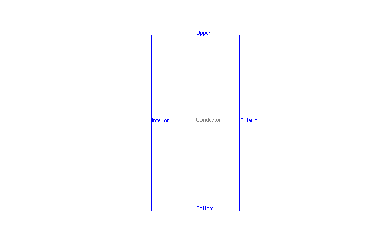
Geometry in axisymmetrical cut

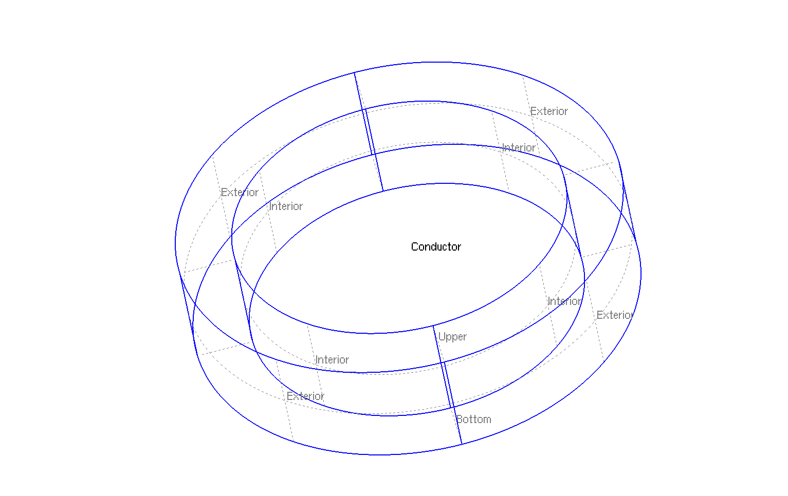
Geometry in three dimensions

The geometrical domains are :

Conductor : the torus, composed by conductive material
Interior and Exterior : interior and exterior of ring (or right and left of rectangle in axisymmetric coordinates \((r,z)\)) correspond to \(\Gamma_R\)
Bottom and Upper : up and bottom of the ring (or up and bottom of the rectangle in axisymmetric coordinates \((r,z)\)) correspond to \(\Gamma_N\)

Symbol

Description

value

unit

\(r_{int}\)

interior radius of torus

\(75e-3\)

\(r_{ext}\)

exterior radius of torus

\(100.2e-3\)

\(z_1\)

half-height of torus

\(25e-3\)

6. Boundary Conditions

We impose the boundary conditions :

Neumann : \(\frac{\partial T}{\partial \mathbf{n}} = 0\) on Interior and Exterior
Robin : \(-k \, \frac{\partial T}{\partial \mathbf{n}} = h \, \left( T - T_c \right)\) on Upper and Bottom

On JSON file, the boundary conditions are writed :

Boundary conditions on JSON file

    "BoundaryConditions":
    {
        "heat":
        {
            "Robin":
            {
                "Interior":
                {
                    "expr1":"h*x:h:x",
                    "expr2":"h*T_c*x:h:T_c:x"
                },
                "Exterior":
                {
                    "expr1":"h*x:h:x",
                    "expr2":"h*T_c*x:h:T_c:x"
                }
            }
        }
    }

7. Weak Formulation

We obtain :

Weak Formulation of Heat Equation in axisymmetric coordinates

\[\small{ \int_{\Omega_c^{axis}}{ k \, \tilde{\nabla} T \cdot \tilde{\nabla} \phi \, r \, drdz } + \int_{\Gamma_R^{axis}}{ h \, T \, \phi \, r \, d\Gamma } = \int_{\Omega_c^{axis}}{ Q \, \phi \, r \, drdz } + \int_{\Gamma_R^{axis}}{ h \, T_c \, \phi \, r \, d\Gamma } }\]

8. Parameters

The parameters of problem are :

On Conductor :

Symbol

Description

Value

Unit

\(Q\)

source term

\(\sigma \, \left( \frac{U}{2\pi \, r} \right)\)

\(U\)

electrical potential

\(1\)

\(Volt\)

\(\sigma\)

electrical conductivity

\(58e6\)

\(S/m\)

\(k\)

thermal conductivity

\(380\)

\(W/m/K\)

\(h\)

convective coefficient

\(8e4\)

\(W/m^2/K\)

\(T_c\)

cooling temperature

\(293\)

\(K\)

On JSON file, the parmeters are writed :

Parameters on JSON file

    "Parameters":
    {
        "h":80000,  // W/m2/K
        "T_c":293,  // K
        "U":1,      // V

        // Constants of analytical solve
        "a":1933.10,    // K
        "b":0.40041,    // K
        "rmax":0.0861910719118454,  // m
        "Tmax":364.446  // K
    }

9. Coefficient Form PDEs

We use the application Coefficient Form PDEs. The coefficient associate to Weak Formulation are :

On Conductor :

Coefficient

Description

Expression

\(c\)

diffusion coefficient

\(r \, k\)

\(f\)

source term

\(- \sigma \left( \frac{U}{2\pi} \right)^2 \frac{1}{r}\)

On JSON file, the coefficients are writed :

CFPDEs coefficients on JSON file

    "Materials":
    {
        "Conductor":
        {
            "k":380,        // W/m/K
            "sigma":58e+6,  // S.m-1
            "heat_c":"k*x:k:x",
            "heat_f":"sigma*(U/2/pi)*(U/2/pi)/x:sigma:U:x"
        }
    }

10. Numeric Parameters

This section show the parameters used to compute the simulation.

Size of mesh : \(0.1 \,mm\)
Element type : \(P1\)
Solver : automatic
Number of CPU core : \(8\)

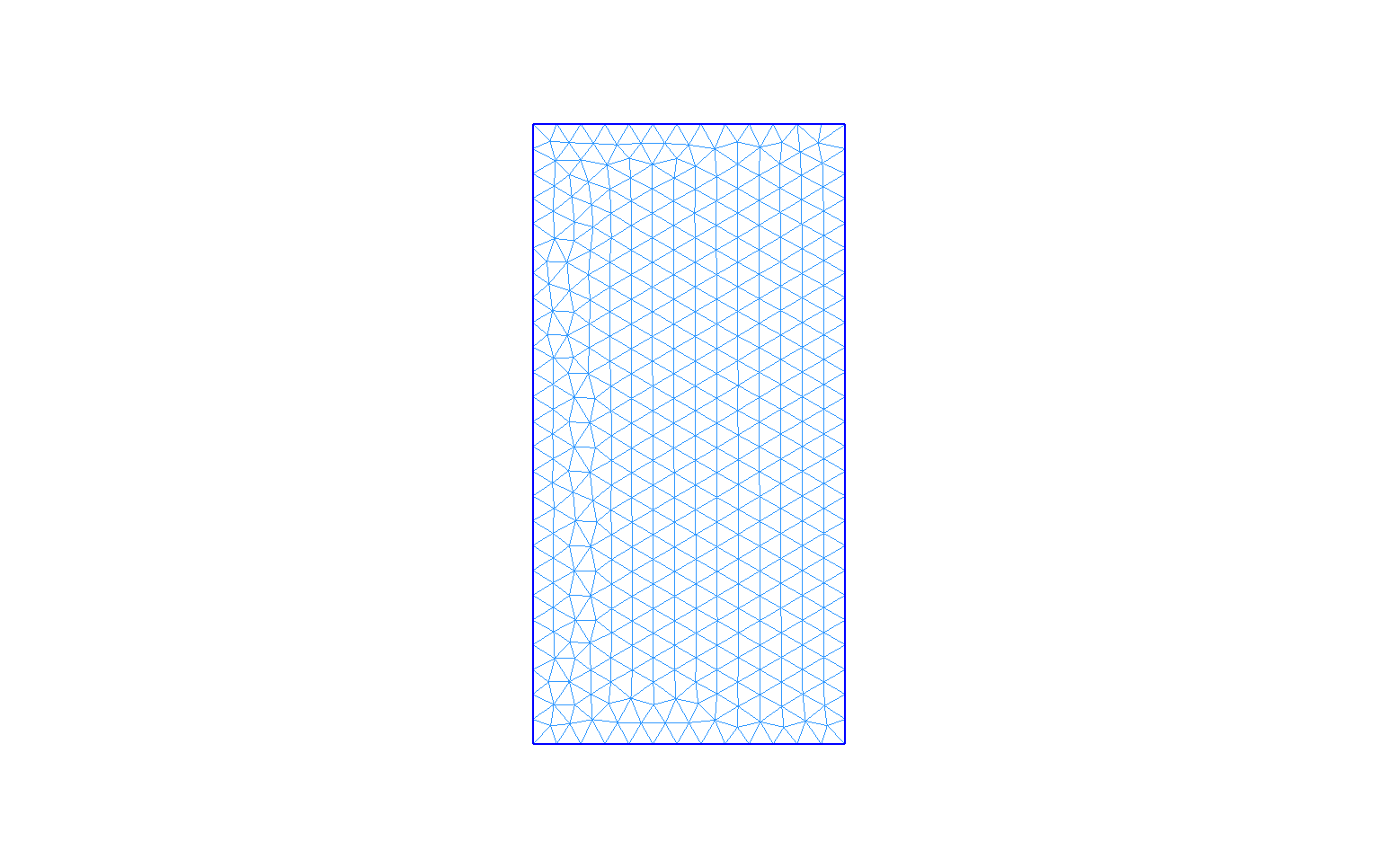
Mesh of Geometry in axisymmetrical (size of mesh \(10 \, mm\))

11. Result

We obtain :

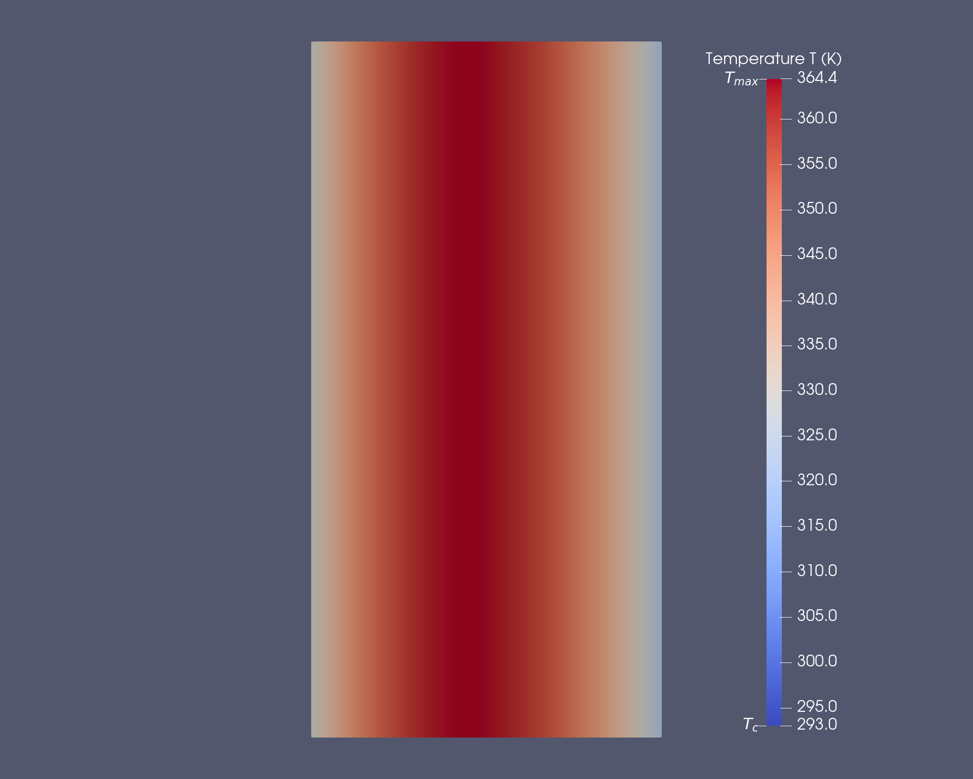
\(T\) \((K)\)

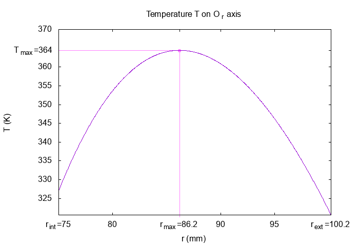
\(T\) \((K)\) on \(Or\) axis

The temperature is constant by \(z\). We can see with the cut, the temperature have a profil of bell. The temperature is less at the cooled interior and exterior than the middle of torus.

12. Validation

12.1. Exact solution

In this section, we compute the exact solution of problem.

The problem is independant of \(z\), thus, the equation (Heat Axis) becomes :

\[ - \frac{1}{r} \frac{\partial \left( r \frac{\partial T}{\partial r} \right)}{\partial r} = \sigma \left( \frac{u}{2\pi \, r} \right)\]

Thus :

\[ T = a \, ln(r) - \frac{\sigma}{2k} \left( \frac{U}{2\pi} \right)^2 \, ln^2(r) + b\]

With \(a\) and \(b\) integrate constants.

With the Robin boundary conditions :

\[ -k \frac{\partial T}{\partial \mathbf{n}} = h(r) \left( T(r) - T_c(r) \right)\]

So :

\[\left\{ \begin{eqnarray*} \left( k+h_{ext} r_{ext} ln(r_{ext}) \right) \, a + h_{ext} r_{ext} b = \frac{\sigma}{2k} \left( \frac{U}{2\pi} \right)^2 ln(r_{ext}) \left( h_{ext} r_{ext} ln(r_{ext})+2k \right) + h_{ext} r_{ext} T_{c \, ext} \\ \left( -k+h_{int} r_{int} ln(r_{int}) \right) \, a + h_{int} r_{int} b = \frac{\sigma}{2k} \left( \frac{U}{2\pi} \right)^2 ln(r_{int}) \left( h_{int} r_{int} ln(r_{int})-2k \right) + h_{int} r_{int} T_{c \, int} \end{eqnarray*} \right.\]

With \(T_{c \, int}=T(r_{int})\), \(T_{c \, ext}=T(r_{ext})\), \(h_{int}=h(r_{int})\) and \(h_{ext}=h(r_{ext})\).

And, with our conditions :

\[\left\{ \begin{eqnarray*} a &=& \frac{\sigma}{2k} \left( \frac{U}{2 \pi} \right)^2 \\ b &=& k \left( \frac{1}{h_{int} r_{int}} + \frac{1}{h_{ext} r_{ext}} \right) + ln(\frac{r_{ext}}{r_{int}}) \end{eqnarray*} \right.\]

The temperature can be right like :

\[ T(r) = - a ln^2(\frac{r}{r_{max}}) + T_{max}\]

With \(T_{max} = T(r_{max})\) the maximal temperature and \(r_{max}\) its input.

And :

\[ r_{max} = e^{\frac{T_{c \, int}-T_{c \, ext} + ac}{2 \, a \, b}}\]

\[ T_{max} = \frac{2 \, a \, k}{h_{int} r_{int} + h_{ext} r_{ext}} \, ln(h_{int} r_{int} + h_{ext} r_{ext}) + \frac{h_{int} r_{int} T_{c \, int} + h_{ext} r_{ext} T_{c \, ext}}{h_{int} r_{int} + h_{ext} r_{ext}} + a \frac{ h_{int} r_{int} ln^2(\frac{r_{int}}{r_{max}}) + h_{ext} r_{ext} ln^2(\frac{r_{ext}}{r_{max}}) }{h_{int} r_{int} + h_{ext} r_{ext}}\]

12.2. Convergence Test

I compute the error between numeric result and theorical solution with differents size of mesh and I obtain :

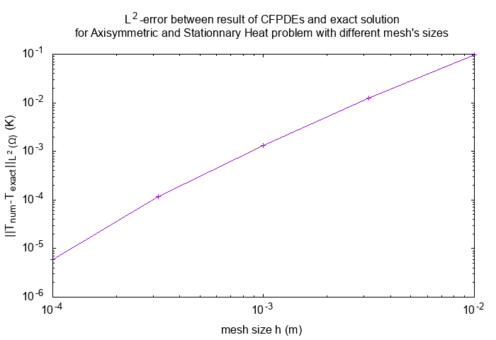
L2-error

Table 1. Table of data
hsize (m)	\(\Vert T_{num} - T_{exact} \Vert_{L^2} (K)\)
1e-2	9.596e-02
3.16e-3	1.229e-02
1e-3	1.313e-03
3.16e-4	1.182e-04
1e-4	5.872e-06

Our implementation of static heat equation in axisymmetrical coordinates converges.

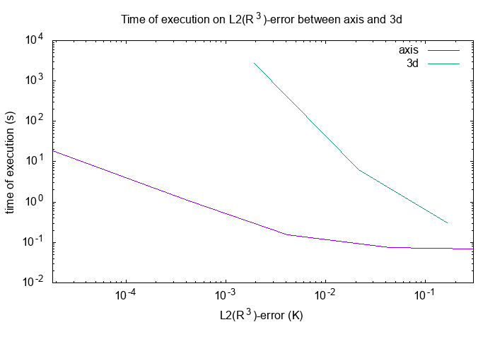
13. Comparison with Three Dimensions

I run the heat problem for axisymmetrical and cartesian cases for different mesh size on the same computer (computer server kelvin) in sequential. I compute the associated L2-error and I recuperates the time of execution.

For axisymmetrical case, I compute the L2-error on \(\mathbb{R}^3\), so :

\[\begin{eqnarray*} ||T_{num}-T_{exact}||_{L^2(\Omega)} &=& \sqrt{ \int \int \int \left( T_{num}-T_{exact} \right)^2 \, r \, dr d\theta dz } \\ &=& \sqrt{2\pi} \sqrt{ \int \int \left( T_{num}-T_{exact} \right) \, r \, dr dz } \end{eqnarray*}\]

I plot the time by L2-error :

time by L2-error

Table 2. Time for axysimmetrical case
L2-error (K)	time (s)
0.3014	6.795e-02
0.04384	7.601e-02
0.004126	1.529e-01
0.0004291	1.075e+00
1.8447e-05	1.831e+01

Table 3. Time for cartesian case
L2-error (K)	time (s)
1.658e-01	3.060e-01s
2.138e-02	6.172e+00s
1.915e-03	2.722e+03s

We can see, for the same precision, the time of cartesian is greater than the axisymmetrical method. For the same problem, the axisymmetrical method is more performant than the cartesian. It’s normal, the axisymmetrical method is a finite element resolution in Two dimensions.