Test Case of Static Elasticity in Axisymmetrical Coordinates
1. Introduction
This page present a test case to validate the implementation of elastic equation with Hooke law without thermal dilatation in static and axisymmetric case in vectorial form.
The result permit, or not, to verify if our method for static elasticity resolution is good.
We inject a function, here \(u=\begin{pmatrix} \frac{e^z}{r} \\ \frac{e^z}{r}\end{pmatrix}\), we inject in equation (Static Elasticity Axis), we recuperate the associated coefficient. We run a simulation with those coefficient and compare the numeric result with the begining function.
2. Run the calculation
The command line to run this case is :
mpirun -np 16 feelpp_toolbox_coefficientformpdes --config-file=elastic.cfg --cfpdes.gmsh.hsize=5e-3
3. Data Files
The case data files are available in Github here :
-
CFG file - Edit the file
-
JSON file - Edit the file
-
GEO file - Edit the file
-
SH file - Edit the file : it serves to compute the same test case but with different mesh sizes.
4. Equation
We solve the elastic equation with Hooke law in static and axisymmetric case (for more detail see section In axisymmetric coordinates).
The differential formulation is :
With :
-
The displacement \(\mathbf{u} = \begin{pmatrix} u_r \\ u_z \end{pmatrix}_{axis}\), the unknow of equation
-
The stress tensor \(\bar{\bar{\sigma}}_{ij} = \lambda \, \delta_{ij} \, \nabla \cdot \mathbf{u} + 2 \, \mu \, \bar{\bar{\epsilon}}_{ij}\) with the tensor of small displacement \(\bar{\bar{\epsilon}}_{ij} = \frac{1}{2} \, \left( \frac{\partial u_{j}}{\partial j} + \frac{\partial u_{i}}{\partial i} \right) \ \text{ for } i,j = x, y, z\) and \(\lambda\) and \(\mu\) the Lamé’s coefficients.
-
The tensor of stiffness \(k\)
-
Volumic Forces \(\mathbf{F}\)
and notations :
-
Divergence of a axisymmetrical tensor : \(\nabla \cdot \bar{\bar{\sigma}} = \begin{pmatrix} \nabla \cdot \bar{\bar{\sigma}}_{r,:} + \frac{\bar{\bar{\sigma}}_{rr} - \bar{\bar{\sigma}}_{\theta \theta}}{r} \\ \nabla \cdot \bar{\bar{\sigma}}_{z,:} + \frac{\bar{\bar{\sigma}}_{rz}}{r} \end{pmatrix}_{axis}\)
-
Scalar produce of a axisymmetrical tensor : \(\bar{\bar{\sigma}} \cdot \mathbf{n} = \begin{pmatrix} \bar{\bar{\sigma}}_{r,:} \cdot \mathbf{n} \\ \bar{\bar{\sigma}}_{r,:} \cdot \mathbf{n} \end{pmatrix} = \begin{pmatrix} \bar{\bar{\sigma}}_{rr} \, n_r + \bar{\bar{\sigma}}_{rz} \, n_z \\ \bar{\bar{\sigma}}_{rz} \, n_r + \bar{\bar{\sigma}}_{zz} \, n_z \end{pmatrix}\)
5. Geometry
The geometry is a torus in cartesian coordinates \((x,y,z)\) or rectangle in axisymmetric coordinates \((r,z)\).
The geometrical domains are :
-
Omega: the torus-
Interior: interior surface ofOmega -
Exterior: exterior surface ofOmega -
Upper: upper ofOmega -
Bottom: bottom ofOmega
-
Symbol |
Description |
value |
unit |
\(r_{int}\) |
interior radius of torus |
\(1\) |
m |
\(r_{ext}\) |
exterior radius of torus |
\(2\) |
m |
\(z_1\) |
half-height of torus |
\(5\) |
m |
We have \(\texttt{Interior} \cup \texttt{Exterior} = \Gamma_{D \hspace{0.05cm} elas}^{axis}\), \(\texttt{Bottom} = \Gamma_{N \hspace{0.05cm} elas}^{axis}\) and \(\texttt{Upper} = \Gamma_{R \hspace{0.05cm} elas}^{axis}\)
6. Boundary Conditions
We impose the boundary conditions :
-
Strong Dirichlet on
Interior,Exterior,BottomandUpper.
On JSON file, the boundary conditions are writed :
    "BoundaryConditions":
    {
        "elastic":
        {
            "Dirichlet":
            {
                "Interior":
                {
                    "expr":"{exp(y)/x,exp(y)/x}:x:y"
                },
                "Exterior":
                {
                    "expr":"{exp(y)/x,exp(y)/x}:x:y"
                },
                "Bottom":
                {
                    "expr":"{exp(y)/x,exp(y)/x}:x:y"
                },
                "Upper":
                {
                    "expr":"{exp(y)/x,exp(y)/x}:x:y"
                }
            }
        }
    }
7. Weak Formulation
We obtain :
8. Solution
We take a function \(u = \begin{pmatrix} \frac{e^z}{r} \\ \frac{e^z}{r} \end{pmatrix}\). For Robin condition we put \(k=\begin{pmatrix} \mu & 0 \\ 0 & \mu \end{pmatrix}\). We inject that on (Static Elasticity Axis) and we obtain :
9. Parameters
The parameters of problem are :
Symbol |
Description |
Value |
Unit |
\(E\) |
Young modulus |
\(2.1e-6\) |
\(Pa\) |
\(v\) |
Poisson’s coefficient |
\(0.33\) |
\(dimensionless\) |
\(\lambda\) |
Lamé’s coefficient |
\(\frac{E \, v}{(1-2 v) \, (1+v)}\) |
\(Pa\) |
\(\mu\) |
Lamé’s coefficient |
\(\frac{E}{2 \, (1+v)}\) |
\(Pa\) |
\(F = \begin{pmatrix} F_r \\ F_z \end{pmatrix}\) |
term source |
\(\begin{pmatrix} \left( \frac{\lambda + \mu}{r} - \mu \right) \frac{e^z}{r} \\ - \left( \frac{\mu}{r^2} + \lambda + 2\mu \right) \frac{e^z}{r} \end{pmatrix}\) |
\(N / m^3\) |
On JSON file, the parmeters are writed :
    "Parameters":
    {
        "E":2.1e6,
        "v":0.33,
	    "lambda":"E*v/(1-2*v)/(1+v):E:v",
        "mu":"E/(2*(1+v)):E:v",
        "Fr":"((lambda+mu)/x-mu)*exp(y)/x:lambda:mu:x:y",
        "Fz":"-(mu/x/x+lambda+2*mu)*exp(y)/x:lambda:mu:x:y"
    }
10. Coefficient Form PDEs
We use the application Coefficient Form PDEs. The coefficients associate to Weak Formulation are :
Coefficient |
Description |
Expression |
\(c\) |
diffusion coefficient |
\(r \mu\) |
\(\gamma\) |
conservative flux source term |
\(\begin{pmatrix} - \lambda \left( r \frac{\partial u_r}{\partial r} + u_r + r \frac{\partial u_z}{\partial z} \right) - \mu \, r \, \frac{\partial u_r}{\partial r} & - \mu \, r \, \frac{\partial u_z}{\partial r} \\ - \mu \, r \, \frac{\partial u_r}{\partial z} & - \lambda \left( r \, \frac{\partial u_r}{\partial r} + u_r + r \, \frac{\partial u_z}{\partial z} \right) - \mu \, r \, \frac{\partial u_z}{\partial z} \end{pmatrix}\) |
\(f\) |
source term |
\(\begin{pmatrix} r F_r - \lambda \frac{\partial u_r}{\partial r} - (\lambda+2\mu) \frac{u_r}{r} - \lambda \frac{\partial u_z}{\partial z} \\ r F_z \end{pmatrix}\) |
On JSON file, the coefficients are writed :
    "Materials":
    {
        "Omega":
        {
            "elastic_c":"x*mu:x:mu",
            "elastic_gamma":"{-lambda*(x*elastic_grad_u_00+elastic_u_0+x*elastic_grad_u_11)-x*mu*elastic_grad_u_00, -x*mu*elastic_grad_u_10, -x*mu*elastic_grad_u_01, -lambda*(x*elastic_grad_u_00+elastic_u_0+x*elastic_grad_u_11)-x*mu*elastic_grad_u_11}:x:lambda:mu:elastic_u_0:elastic_grad_u_00:elastic_grad_u_01:elastic_grad_u_10:elastic_grad_u_11",
            "elastic_f":"{x*Fr-lambda*elastic_grad_u_00-(lambda+2*mu)*elastic_u_0/x-lambda*elastic_grad_u_11, x*Fz}:x:Fr:Fz:mu:lambda:elastic_u_0:elastic_grad_u_00:elastic_grad_u_01:elastic_grad_u_11"
        }
    }
11. Validation
We compute the L2-error between numerical solution and begining function with different size of mesh :
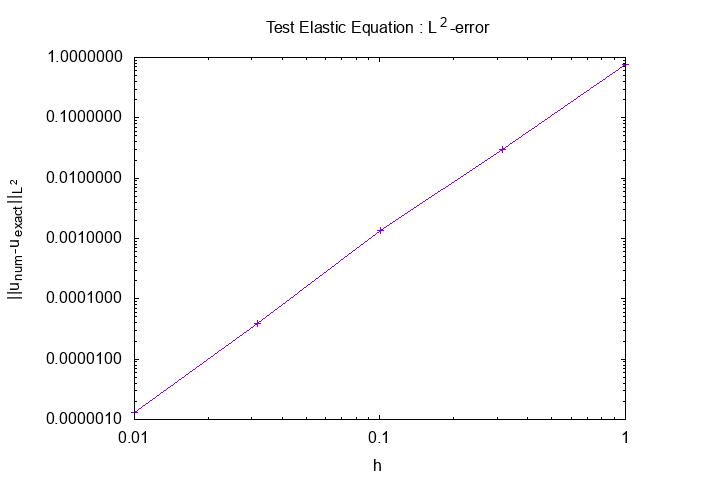
\(L^2-error\)
|
The method converge with polynomial order, the L2-error form a right in xy logarithmic scale.
Conclusion : We trust on this method to solve the static elasticity equation (Static Elasticity Axis).