Axisymmetrical Case

1. T-A Formulation

T-A Formulation

\[\text{(T-A)}\left\{ \begin{matrix} \nabla\times\left(\frac{1}{\mu}\nabla\times\textbf{A}\right) &=& \nabla\times\textbf{T} \text{ on } \Omega & \text{(A-form)} \\ \nabla \times \left(\rho\nabla\times\textbf{T} \right) &=& -\frac{\partial (\nabla\times\textbf{A})}{\partial t} \text{ on } \Omega_c & \text{(T-form)} \\ \mathbf{A} \times \mathbf{n} &=& 0 \text{ on } \Gamma_D & \text{(D)} \\ \left( \nabla \times \mathbf{A} \right) \times \mathbf{n} &=& 0 \text{ on } \Gamma_N & \text{(N)} \end{matrix} \right.\]

2. Differential Formulation

In this section, we will express the T-A Formulation on a geometry in axisymmetric coordinates.

We note \(\Omega^{axis}\), \(\Omega^{axis}_c\), \(\Gamma^{axis}\), \(\Gamma_D^{axis}\), \(\Gamma_N^{axis}\) and \(\Gamma_c^{axis}\) the representation of \(\Omega\), \(\Omega_c\), \(\Gamma\), \(\Gamma_D\), \(\Gamma_N\) and \(\Gamma_c\) in axisymmetric coordinates.

We note \(u = \begin{pmatrix} u_r \\ u_{\theta} \\ u_z \end{pmatrix}_{cyl}\) the coordinates of \(u \in \mathbb{R}^3\) in cylindrical base.

We note \(\mathbf{n}^{axis} = \begin{pmatrix} n^{axis}_r \\ n^{axis}_z \end{pmatrix}_{cyl}\) the exterior normal of \(\Gamma^{axis}\) on \(\Omega^{axis}\).

First, for the A-formulation we will use the same changes as in the Atheta Axisymmetric case. We have \(\mathbf{B} = \begin{pmatrix} B_r(r,z) \\ 0 \\ B_z(r,z) \end{pmatrix}_{cyl}\) and \(\mathbf{A}= \begin{pmatrix} 0 \\ A_{\theta}(r,z) \\ 0 \end{pmatrix}_{cyl}\) and :

A Formulation

\[ -\frac{1}{\mu}\Delta A_\theta + \frac{1}{\mu r^2}A_\theta =J\text{ on }\Omega^{axis} \hspace{2cm} \text{(A Axis)}\]

On the other hand, due to the aspect ratio between the height and the width of the coated conductor, the T-A formulation uses a thin strip approximation of the tapes, reducing the superconducting domain to a thin sheet.

Figure 1. Bounded universe with superconductive layers and surrounding medium.

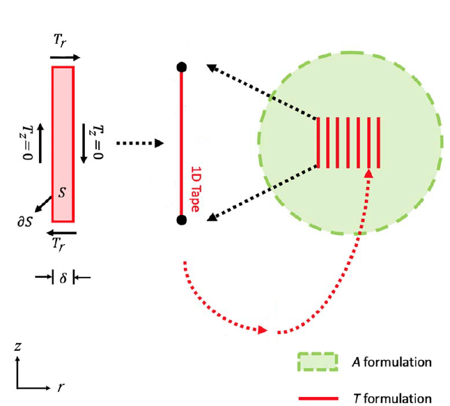
The current is restricted to flow within this sheet, and \(T\) is reduced to the component perpendicular to the tape. In axisymmetrical coordinates, the HTS tape is reduced to a 1D vertical line element and \(J=\nabla\times T\) becomes :

\[ J_\theta = \frac{\partial T_r}{\partial z}\]

Then when using the faraday law to have the T-formulation, the equation can be reduced to :

\[-\frac{\partial E_\theta}{\partial z} = -\frac{\partial B_r}{\partial t}\]

We can replace \(E_\theta\) using \(E=\rho J\) and \(B_r\) with \(-\frac{\partial A_\theta}{\partial z}\) :

\[-\frac{\partial (\rho J_\theta)}{\partial z} = \frac{\partial (\partial_z A_\theta)}{\partial t}\]

As \(T = \begin{pmatrix} T_r(r,z) \\ 0 \\ 0 \end{pmatrix}_{cyl}\), we have \(\frac{\partial \rho J_\theta}{\partial z} =\rho \frac{\partial^2 T}{\partial z^2}\) and the equation becomes :

T Formulation

\[-\begin{pmatrix} 0 & 0 \\ 0 & \rho \end{pmatrix} \Delta T_r = \frac{\partial (\partial_z A_\theta)}{\partial t} \text{ on }\Omega_c^{axis} \hspace{2cm} \text{(T Axis)}\]

We replace \(J\) in the A-formulation by \(\frac{\partial T_r}{\partial z}\).

To conclude, the T-A Formulation becomes :

T-A Formulation in axisymmetric coordinates

\[\text{(TA Axis)} \left\{ \begin{matrix} -\frac{1}{\mu}\Delta A_\theta + \frac{1}{\mu r^2}A_\theta =\frac{\partial T_r}{\partial z}& \text{ on } \Omega^{axis} &\text{(A Axis)} \\ -\begin{pmatrix} 0 & 0 \\ 0 & \rho \end{pmatrix} \Delta T_r = \frac{\partial (\partial_z A_\theta)}{\partial t}& \text{ on } \Omega_c^{axis} & \text{(T Axis)} \\ A_{\theta} = 0 & \text{ on } \Gamma_D^{axis} & \text{(D Axis)} \\ \frac{\partial A_{\theta}}{\partial \mathbf{n}^{axis}} = 0 & \text{ on } \Gamma_N^{axis} & \text{(N Axis)} \end{matrix} \right.\]

With \(\Delta A_\theta = \frac{\partial^2 A_\theta}{\partial z^2} + \frac{1}{r} \frac{\partial \left( r \frac{\partial A_\theta}{\partial r} \right)}{\partial r} \)

2.1. Transport Current

The boundary conditions at the edge of the 1D superconducting layer for \(T\) can be obtained by integrating the current density \(J\) over the cross-section of the layer which is equal to the transport current in the tape :

\[ I= \iint_{S}{ J dS} =\iint_{S}{ \nabla\times T dS} = \oint_{\partial S } T dr \hspace{1cm} \text{(Transport Current)}\]

As the component of \(T\) parallel to the layer is zero, \(I\) becomes :

\[ I= (T_1 -T_2)\delta \hspace{1cm} \text{(Transport Current)}\]

with \(\delta\) being the thickness of the superconducting tape and \(T_1\) and \(T_2\), the potentials at the extremities of the 1D layer.

Therefore, by modifying \(T_1\) and \(T_2\), we can express the transport current.

3. Weak Formulation

The weak formulation of equation (TA Axis) in two dimensions can be expressed as follows :

We multiply the equation (A Axis) by \(\phi \in H^1(\Omega)\) and integrate it on \(\Omega\) :

\[ \int_{\Omega}{ - \frac{1}{\mu} \Delta A_\theta + \frac{1}{\mu r^2}A_\theta \cdot \phi \ dxdydz} = \int_{\Omega_c}{ \frac{\partial T_r}{\partial z} \cdot \phi \ dxdydz} \hspace{1cm} \text{(Weak A Axis)}\]

By Formula of Green :

\[\scriptsize{ \int_{\Omega}{ \frac{1}{\mu} \nabla A_\theta \cdot \nabla \phi \ dxdydz } - \int_{\Gamma}{ \frac{1}{\mu} \frac{\partial A_\theta}{\partial \mathbf{n}} \cdot \phi \ d\Gamma} + \int_{\Omega}{\frac{1}{\mu r^2} A_\theta \cdot \phi \ dxdydz} = \int_{\Omega_c}{ \frac{\partial T_r}{\partial z} \cdot\phi \ dxdydz } \hspace{1cm} \text{(Disc A Axis)} }\]

We switch to axisymmetrical coordinates :

\[\scriptsize{ \int_{\Omega^{axis}}{ \frac{1}{\mu} \tilde\nabla A_\theta \cdot \tilde\nabla \phi \ rdrdz } - \int_{\Gamma^{axis}}{ \frac{1}{\mu} (\tilde\nabla A_\theta\cdot n^{axis}) \cdot \phi \ d\Gamma} + \int_{\Omega^{axis}}{\frac{1}{\mu r^2} A_\theta \cdot \phi \ rdrdz} = \int_{\Omega^{axis}_c}{ \frac{\partial T_r}{\partial z} \cdot\phi \ rdrdz } }\]

With \(\tilde{\nabla} = \begin{pmatrix} \partial_r \\ \partial_{\theta} \\ \partial_z \end{pmatrix}_{cyl}\)

\[\scriptsize{ \int_{\Omega^{axis}}{ \frac{r}{\mu} \tilde\nabla A_\theta \cdot \tilde\nabla \phi \ drdz } - \int_{\Gamma_D^{axis}}{ \frac{r}{\mu} (\tilde\nabla A_\theta\cdot n^{axis}) \cdot \phi \ d\Gamma}- \int_{\Gamma_N^{axis}}{ \frac{r}{\mu} (\tilde\nabla A_\theta\cdot n^{axis}) \cdot \phi \ d\Gamma} + \int_{\Omega^{axis}}{\frac{1}{\mu r} A_\theta \cdot \phi \ drdz} += \int_{\Omega^{axis}_c}{ \frac{\partial T_r}{\partial z} \cdot\phi \ rdrdz } }\]

We impose the boundary conditions :

Dirichlet : \(A_{\theta} = 0\) on \(\Gamma_D^{axis}\) (D Axis)
Neumann : \(\frac{\partial A_{\theta}}{\partial n} = 0\) on \(\Gamma_N^{axis}\) (N Axis)

So, the weak formulation is :

\[\scriptsize{ \int_{\Omega^{axis}}{ \frac{r}{\mu} \tilde\nabla A_\theta \cdot \tilde\nabla \phi \ drdz } + \int_{\Omega^{axis}}{\frac{1}{\mu r} A_\theta \cdot \phi \ drdz} = \int_{\Omega^{axis}_c}{ \frac{\partial T_r}{\partial z} \cdot\phi \ rdrdz } \text{ for } \phi \in H^1(\Omega) }\]

Then we multiply the equation (T Axis) by \(\varphi \in H^1(\Omega_c)\) and integrate it on \(\Omega_c\) :

\[ \int_{\Omega_c}{ - \begin{pmatrix} 0 & 0 \\ 0 & \rho \end{pmatrix} \Delta T_r \cdot \varphi \ dxdydz} = \int_{\Omega_c}{ \frac{\partial (\partial_z A_\theta)}{\partial t} \cdot \varphi \ dxdydz} \hspace{1cm} \text{(Weak T Axis)}\]

By Formula of Green :

\[\scriptsize{ \int_{\Omega_c}{ \begin{pmatrix} 0 & 0 \\ 0 & \rho \end{pmatrix} \nabla T_r \cdot \nabla \varphi \ dxdydz } - \int_{\Gamma}{ \begin{pmatrix} 0 & 0 \\ 0 & \rho \end{pmatrix} \frac{\partial T_r}{\partial \mathbf{n}} \cdot \varphi \ d\Gamma} = \int_{\Omega_c}{ \frac{\partial (\partial_z A_\theta)}{\partial t} \cdot\varphi \ dxdydz } \hspace{1cm} \text{(Disc T Axis)} }\]

We switch to axisymmetrical coordinates :

\[\scriptsize{ \int_{\Omega^{axis}_c}{ \begin{pmatrix} 0 & 0 \\ 0 & \rho \end{pmatrix} \tilde\nabla T_r \cdot \tilde\nabla \varphi \ rdrdz } - \int_{\Gamma^{axis}}{ \begin{pmatrix} 0 & 0 \\ 0 & \rho \end{pmatrix} (\tilde\nabla T_r\cdot n^{axis}) \cdot \varphi \ d\Gamma} = \int_{\Omega^{axis}_c}{ \frac{\partial \partial_z}{\partial t} \cdot\varphi \ rdrdz } }\]

With \(\tilde{\nabla} = \begin{pmatrix} \partial_r \\ \partial_{\theta} \\ \partial_z \end{pmatrix}_{cyl}\)

\[\scriptsize{ \int_{\Omega^{axis}_c}{ \begin{pmatrix} 0 & 0 \\ 0 & \rho \end{pmatrix} \tilde\nabla T_r \cdot \tilde\nabla \varphi \ rdrdz } - \int_{\Gamma_D^{axis}}{ \begin{pmatrix} 0 & 0 \\ 0 & \rho \end{pmatrix} (\tilde\nabla T_r\cdot n^{axis}) \cdot \varphi \ d\Gamma}- \int_{\Gamma_N^{axis}}{\begin{pmatrix} 0 & 0 \\ 0 & \rho \end{pmatrix} (\tilde\nabla T_r\cdot n^{axis}) \cdot \varphi \ d\Gamma} =\int_{\Omega^{axis}_c}{ \frac{\partial (\partial_z A_\theta)}{\partial t} \cdot \varphi \ rdrdz} }\]

We impose the boundary conditions :

Dirichlet : \(T_r = 0\) on \(\Gamma_D^{axis}\) (D Axis)
Neumann : \(\frac{\partial T_r}{\partial n} = 0\) on \(\Gamma_N^{axis}\) (N Axis)

So, the weak formulation is :

\[\scriptsize{ \int_{\Omega^{axis}_c}{ \begin{pmatrix} 0 & 0 \\ 0 & \rho \end{pmatrix} \tilde\nabla T_r \cdot \tilde\nabla \varphi \ drdz } = \int_{\Omega^{axis}_c}{ \frac{\partial (\partial_z A_\theta)}{\partial t} \cdot\varphi \ rdrdz } \text{ for } \varphi \in H^1(\Omega_c) }\]

Finally we have :

Weak formulation of T-A Formulation in axisymmetric coordinates

\[\scriptsize{ \text{(Weak TA Axis)} \left\{ \begin{eqnarray*} \int_{\Omega^{axis}}{ \frac{r}{\mu} \tilde\nabla A_\theta \cdot \tilde\nabla \phi \ drdz } + \int_{\Omega^{axis}}{\frac{1}{\mu r} A_\theta \cdot \phi \ drdz} = \int_{\Omega^{axis}_c}{ \frac{\partial T_r}{\partial z} \cdot\phi \ rdrdz } \\ \int_{\Omega^{axis}_c}{ \begin{pmatrix} 0 & 0 \\ 0 & \rho \end{pmatrix} \tilde\nabla T_r \cdot \tilde\nabla \varphi \ drdz } = \int_{\Omega^{axis}_c}{ \frac{\partial (\partial_z A_\theta}{\partial t} \cdot\varphi \ rdrdz }\\ \text{for } \phi \in H^1(\Omega) \text{ and } \varphi \in H^1(\Omega_c) \end{eqnarray*} \right. }\]

4. Time Discretization

In this subsection, we use the time discretization by backward Euler method on the (Weak T-A Axi).

We discretize in time the problem with the time step \(\Delta t\).

We note \(f^n(\mathbf{x}) = f(n\Delta t, \mathbf{x})\), for \(n \in \mathbb{N}\).

We have the approximation with backward Euler method : \(\frac{\partial (\partial_z A_\theta)}{\partial t} \approx \frac{(\partial_z A_\theta)^{n+1}-(\partial_z A_\theta)^n}{\Delta t}\).

The equations (Weak A Axi) becomes :

Time Discretization of T-A Formulation in axisymmetric

\[\scriptsize{ \text{(Disc TA Axis)}\begin{cases} \int_{\Omega^{axis}}{ \frac{r}{\mu} \tilde\nabla A_\theta^{n+1} \cdot \tilde\nabla \phi \ drdz } + \int_{\Omega^{axis}}{\frac{1}{\mu r} A_\theta^{n+1} \cdot \phi \ drdz} = \int_{\Omega^{axis}_c}{ \frac{\partial T_r^{n+1}}{\partial z} \cdot\phi \ rdrdz } \\ \int_{\Omega^{axis}_c}{ \begin{pmatrix} 0 & 0 \\ 0 & \rho \end{pmatrix} \tilde\nabla T_r^{n+1} \cdot \tilde\nabla \varphi \ drdz } = \int_{\Omega^{axis}_c}{ \frac{ (\partial_z A_\theta)^{n+1} - (\partial_z A_\theta)^{n}}{\Delta t} \cdot\varphi \ rdrdz }\\ \end{cases}}\]

5. Homogeneous Axisymmetrical Case

The homogenization technique is modeling a stack of HTS tapes as a homogeneous anisotropic bulk.

Figure 2. T–A homogeneous approach. The stack is transformed in a bulk.

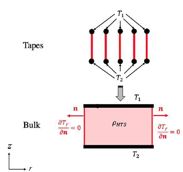
The bulk represent a densely packed stack of 1D superconducting layers. The A-formulation is defined on the entire domain , but the T-formulation is only defined on the superconducting material.

5.1. Differential Formulation

In this section, we will express the T-A Formulation on a geometry in homogeneous axisymetric coordinates.

First, for the A-formulation, we will use a scaled current density approximation :

\[ J_s = \frac{\delta}{\Lambda} J_\theta\]

where \(\delta\) is the thickness of a tape, \(\Lambda\) the space between two tapes and \(J_\theta = \partial T_r/\partial z\).

The A-formulation becomes :

A Formulation

\[ -\frac{1}{\mu}\Delta A_\theta + \frac{1}{\mu r^2}A_\theta =\frac{\delta}{\Lambda} \frac{\partial T_r}{\partial z} \text{ on }\Omega^{axis} \hspace{2cm} \text{(A Axis)}\]

On the other hand, the T-formulation is unaffected by the homogeneous method :

T Formulation

\[-\begin{pmatrix} 0 & 0 \\ 0 & \rho \end{pmatrix} \Delta T_r = \frac{\partial (\partial_z A_\theta)}{\partial t} \text{ on }\Omega_c^{axis} \hspace{2cm} \text{(T Axis)}\]

The T-A Formulation becomes :

T-A Formulation in axisymmetric coordinates

\[\text{(TA Hom Axis)} \left\{ \begin{matrix} -\frac{1}{\mu}\Delta A_\theta + \frac{1}{\mu r^2}A_\theta =\frac{\delta}{\Lambda}\frac{\partial T_r}{\partial z} & \text{ on } \Omega^{axis} &\text{(A Axis Hom)} \\ -\begin{pmatrix} 0 & 0 \\ 0 & \rho \end{pmatrix} \Delta T_r = \frac{\partial (\partial_z A_\theta)}{\partial t} & \text{ on } \Omega_c^{axis} & \text{(T Axis Hom)} \\ A_{\theta} = 0 & \text{ on } \Gamma_D^{axis} & \text{(D Axis)} \\ \frac{\partial A_{\theta}}{\partial \mathbf{n}^{axis}} = 0 & \text{ on } \Gamma_N^{axis} & \text{(N Axis)} \end{matrix} \right.\]

With \(\Delta A_\theta = \frac{\partial^2 A_\theta}{\partial z^2} + \frac{1}{r} \frac{\partial \left( r \frac{\partial A_\theta}{\partial r} \right)}{\partial r} \)

5.2. Transport Current

The boundary conditions at the edge of the 1D superconducting layer for \(T\) are still obtained by integrating the current density \(J\) over the cross-section of the layer which is equal to the transport current in the tape. These boundary conditions are to be appied of the edges of the bulk corresponding to the extremities of the tapes. Additionally, the boundary conditions on the side edges of the bulk are Neumann boundary conditions :

\[ \frac{\partial T_r}{\partial n}=0\]

5.3. Weak Formulation

The weak formulation of equation (TA Axis) in axisymmetric coordinates can be expressed as follows :

Weak formulation of T-A Formulation in axisymmetric coordinates

\[\scriptsize{ \text{(Weak TA Hom Axis)} \left\{ \begin{eqnarray*} \int_{\Omega^{axis}}{ \frac{r}{\mu} \tilde\nabla A_\theta \cdot \tilde\nabla \phi \ drdz } + \int_{\Omega^{axis}}{\frac{1}{\mu r} A_\theta \cdot \phi \ drdz} = \int_{\Omega^{axis}_c}{ \frac{\delta}{\Lambda}\frac{\partial T_r}{\partial z} \cdot\phi \ rdrdz } \\ \int_{\Omega^{axis}_c}{ \begin{pmatrix} 0 & 0 \\ 0 & \rho \end{pmatrix} \tilde\nabla T_r \cdot \tilde\nabla \varphi \ drdz } = \int_{\Omega^{axis}_c}{ \frac{\partial (\partial_z A_\theta)}{\partial t} \cdot\varphi \ rdrdz }\\ \text{for } \phi \in H^1(\Omega) \text{ and } \varphi \in H^1(\Omega_c) \end{eqnarray*} \right. }\]

5.4. Time Discretization

In this subsection, we use the time discretization by backward Euler method on the (Weak T-A Axi).

We discretize in time the problem with the time step \(\Delta t\).

We note \(f^n(\mathbf{x}) = f(n\Delta t, \mathbf{x})\), for \(n \in \mathbb{N}\).

We have the approximation with backward Euler method : \(\frac{\partial (\partial_z A_\theta)}{\partial t} \approx \frac{\partial_z A_\theta^{n+1}-\partial_z A_\theta^n}{\Delta t}\).

The equations (Weak A Axi) becomes :

Time Discretization of T-A Formulation in axisymmetric

\[\scriptsize{ \text{(Disc TA Hom Axis)}\begin{cases} \int_{\Omega^{axis}}{ \frac{r}{\mu} \tilde\nabla A_\theta^{n+1} \cdot \tilde\nabla \phi \ drdz } + \int_{\Omega^{axis}}{\frac{1}{\mu r} A_\theta^{n+1} \cdot \phi \ drdz} = \int_{\Omega^{axis}_c}{ \frac{\delta}{\Lambda}\frac{\partial T_r^{n+1}}{\partial z} \cdot\phi \ rdrdz } \\ \int_{\Omega^{axis}_c}{ \begin{pmatrix} 0 & 0 \\ 0 & \rho \end{pmatrix} \tilde\nabla T_r^{n+1} \cdot \tilde\nabla \varphi \ drdz } = \int_{\Omega^{axis}_c}{ \frac{ (\partial_z A_\theta)^{n+1} - (\partial_z A_\theta)^{n}}{\Delta t} \cdot\varphi \ rdrdz }\\ \end{cases}}\]

6. References

Real-time simulation of large-scale HTS systems: multi-scale and homogeneous models using the T–A formulation, Edgar Berrospe-Juarez et al 2019 Supercond. Sci. Technol. 32 065003, PDF