Test Case of Magnetostatic with Saddle-Point Formulation on One Torus

1. Introduction

This is the test case of Maxwell Quasi Static Problem with the A-V Formulation and Gauge Condition on a torus geometry surrounded by air for the stationary case.

2. Run the Calculation

The command line to run this case is :

    feelpp_toolbox_coefficientformpdes --config-file=magnetostatic_saddle.cfg --cfpdes.gmsh.hsize=5e-3

This case is run with the latest version 109 of Feelpp.

3. Data Files

The case data files are available in Github here :

CFG file - Edit the file
JSON file - Edit the file
GEO file - Edit the file

4. Equation

The domain \(\Omega\) is composed of the conductor \(\Omega_c\) and non conducting materials \(\Omega/\Omega_c\) where \(\mathbf{J} = 0\), like the air for example. \(\Gamma = \partial \Omega\) is the bound of \(\Omega\), decomposed in \(\Gamma_D\) with Dirichlet boundary condition and \(\Gamma_N\) with Neumann boundary condition, such that \(\Gamma = \Gamma_D \cup \Gamma_N\).

We introduce :

Magnetic potential field \(\mathbf{A}\) : the magnetic field is \(\textbf{B} = \nabla \times \textbf{A}\)
Electric potential scalar : \(\nabla V = - \textbf{E}\)

We have the conditions :

\(\nabla \cdot \mathbf{A} = 0\)

We want to resolve the electromagnetic problem ( with \(\mathbf{A}\), \(p\) and \(V\) as the unknowns) :

A-V Saddle-Point Formulation in Stationary Case

\[\text{(Magstat Saddle-Point)} \left\{ \begin{matrix} \nabla \times \left( \frac{1}{\mu} \nabla \times \textbf{A} \right) + \nabla p + \sigma \nabla V &=& 0 &\text{ on } \Omega & \text{(AV-1)} \\ \nabla \cdot \textbf{A}&=&0 &\text{ on } \Omega & \text{(Gauge)} \\ \nabla \cdot \left( \sigma \nabla V \right) &=& 0 &\text{ on } \Omega_c & \text{(AV-2)} \\ \end{matrix} \right.\]

With :

\(\sigma\) : electric conductivity \(S/m\)
\(\mu\) : electric permeability \(kg/A^2/S^2\)

(See A-V Saddle-Point Formulation).

5. Geometry

The geometry is a quarter of a conducting torus, surrounded by air.

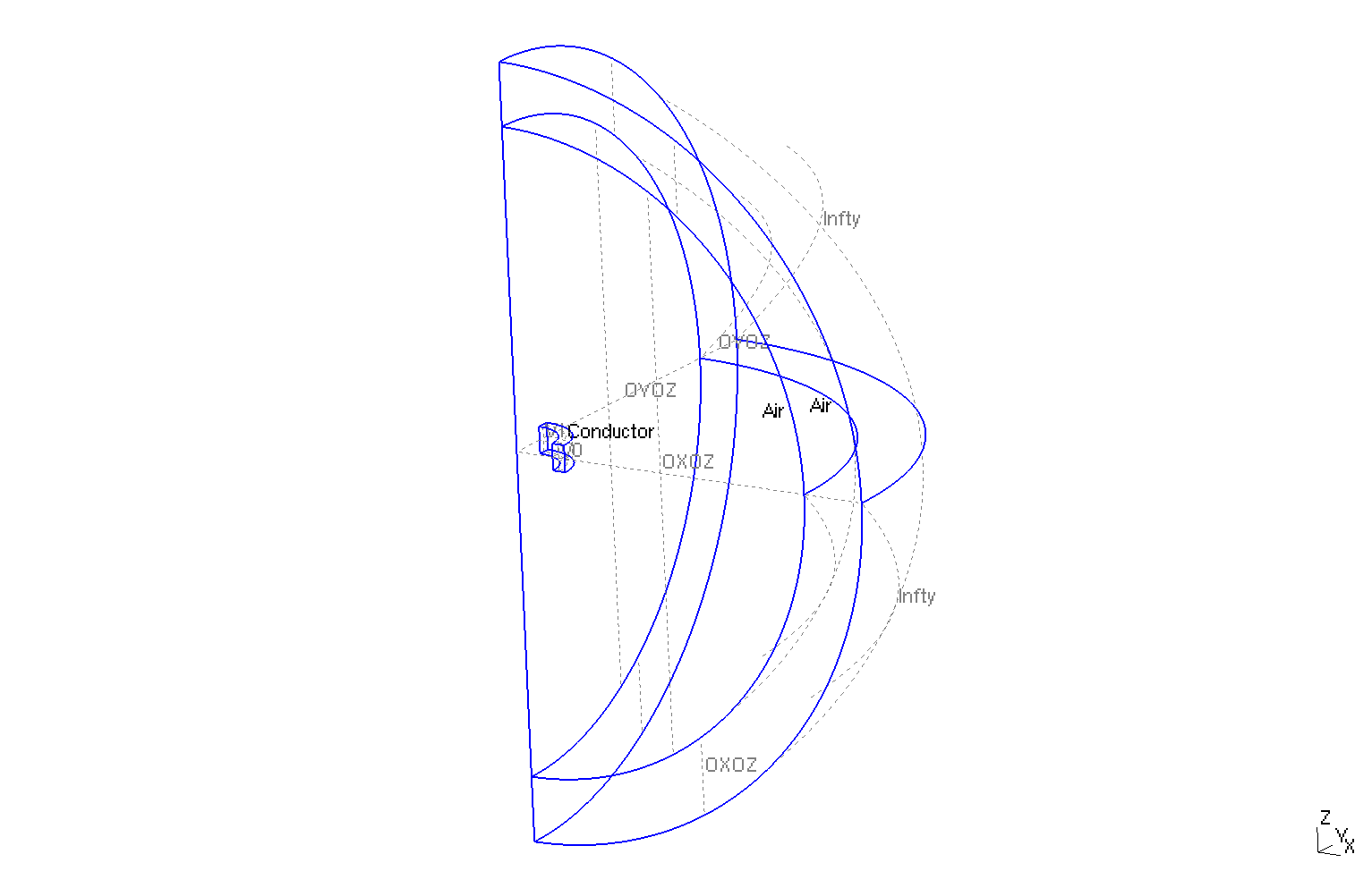
Geometry

The geometrical domains are :

Conductor : the torus, composed by a conductor
- V0 : entrance of electrical potential
- V1 : exit of electrical potential
Air : the air surrounding Conductor
- OXOZ : \(OxOz\) plan
- OYOZ : \(OyOz\) plan
- Infty : the rest of Air 's bound

Symbol

Description

value

unit

\(r_{int}\)

interior radius of torus

\(75e-3\)

\(r_{ext}\)

exterior radius of torus

\(100.2e-3\)

\(z_1\)

half-height of torus

\(25e-3\)

\(r_{infty}\)

radius of infty border

\(5*r_{ext}\)

6. Boundary Conditions

The Dirichlet boundary conditions imposed are :

For \(V\) equation :
- On V0 : \(V=0\)
- On V1 : \(V = \frac{1}{4}\)
For \(\mathbf{A}\) :
- On OXOZ and V0 : \(A_x = A_z = 0\), we want \(\mathbf{A}\) orthogonal to OXOZ and V0
- On OYOZ and V1 : \(A_y = A_z = 0\), we want \(\mathbf{A}\) orthogonal to OYOZ and V1
- Infty : We approximate the problem, Infty is the physical infty so \(\mathbf{B}=0\) at Infty thus \(\mathbf{A} = 0\)
For \(p\) :
- On OXOZ and V0 : \(p = 0\)
- On OYOZ and V1 : \(p = 0\)
- Infty : \(p = 0\)

On JSON file, the boundary conditions are written :

Boundary conditions on JSON file

    "BoundaryConditions":
    {
        "magnetic":
        {
            "Dirichlet":
            {
                "boundary":
                {
                    "markers":["Infty"],
                    "expr":"{0,0,0}"
                },
                "mydir_x":
                {
                    "markers":["V0","OXOZ"],
                    "expr":"{0,0,0}"
                },

                "mydir_y":
                {
                    "markers":["V1","OYOZ"],
                    "expr":"{0,0,0}"
                },
                "mydir_z":
                {
                    "markers":["V0","OXOZ","V1","OYOZ"],
                    "expr":"{0,0,0}"
                }
            }
        },
        "constraint":
        {
            "Dirichlet":
            {
                "boundary":
                {
                    "markers":["Infty"],
                    "expr":"0"
                },
                "mydir_x":
                {
                    "markers":["V0","OXOZ"],
                    "expr":"0"
                },

                "mydir_y":
                {
                    "markers":["V1","OYOZ"],
                    "expr":"0"
                },
                "mydir_z":
                {
                    "markers":["V0","OXOZ","V1","OYOZ"],
                    "expr":"0"
                }
            }
        },
        "electric":
        {
            "Dirichlet":
            {
                "V0":
                {
                    "markers":["V0"],
                    "expr":"V0:V0"
                },
                "V1":
                {
                    "markers":["V1"],
                    "expr":"V1:V1"
                }
            }
        }
    },

7. Weak Formulation

Weak Formulation

\[\scriptsize{ \text{(Weak Magstat Saddle-Point)} \\ \left\{ \begin{eqnarray*} \int_{\Omega}{ \frac{1}{\mu} \nabla \times \textbf{A} \cdot \nabla \times \phi \ dxdydz } &=& - \int_{\Omega}{ \nabla p \cdot \phi \ dxdydz } - \int_{\Omega_c}{ \sigma \nabla V \cdot\phi \ dxdydz } \quad\text{(Weak AV1)} \\ \int_{\Omega_c}{\sigma \nabla V \cdot \nabla \mathbf{\psi}} &=& 0 \quad\text{(Weak AV-2)}\\ &&\forall \phi \in H^{curl}(\Omega) \text{ and } \forall \mathbf{\psi} \in H^{1}(\Omega_c) \end{eqnarray*} \right. }\]

8. Parameters

The parameters of the problem are :

On Conductor :

Symbol

Description

Value

Unit

\(V0\)

scalar electrical potential on V0

\(0\)

\(Volt\)

\(V1\)

scalar electrical potential on V1

\(\frac{1}{4}\)

\(Volt\)

\(\sigma\)

electrical conductivity

\(58e6\)

\(S/m\)

\(\mu=\mu_0\)

magnetic permeability of vacuum

\(4\pi.10^{-7}\)

\(kg \, m / A^2 / S^2\)

On Air :

Symbol

Description

Value

Unit

\(\mu=\mu_0\)

magnetic permeability of vacuum

\(4\pi.10^{-7}\)

\(kg \, m / A^2 / S^2\)

On JSON file, the parameters are written :

Parameters on JSON file

    "Parameters":
    {
        "V0":0,
        "V1":"1/4*1",
        "sigma":58e6,
        "mu":"4*pi*1e-7"
    },

9. Coefficient Form PDEs

The Feelpp toolboxe Coefficient Form PDEs is used here. The coefficients associated to the Weak Formulation are :

On Conductor :

Coefficient

Description

Expression

magnetic_zeta

curlcurl coefficient

\(\frac{1}{\mu}\)

magnetic_f

source term

\(-\nabla p - \sigma \nabla V \)

electric_c

damping or mass coefficient

\(\sigma\)

constraint_gamma

conservative flux source term

\(\mathbf{A}\)

On Air :

Coefficient

Description

Expression

magnetic_zeta

curlcurl coefficient

\(\frac{1}{\mu}\)

magnetic_f

source term

\(-\nabla p\)

constraint_gamma

conservative flux source term

\(\mathbf{A}\)

On JSON file, the coefficients are written :

CFPDEs coefficients on JSON file

    "Materials":
    {
        "Conductor":
        {
            "magnetic_zeta":"1/mu:mu",
            "magnetic_f":"{-constraint_grad_p_0-sigma*electric_grad_V_0,-constraint_grad_p_1-sigma*electric_grad_V_1,-constraint_grad_p_2-sigma*electric_grad_V_2}:sigma:electric_grad_V_0:electric_grad_V_1:electric_grad_V_2:constraint_grad_p_0:constraint_grad_p_1:constraint_grad_p_2",

            "electric_c":"sigma:sigma",
            "constraint_gamma":"{magnetic_A_0,magnetic_A_1,magnetic_A_2}:magnetic_A_0:magnetic_A_1:magnetic_A_2"
        },
        "Air":
        {
            "physics":["magnetic","constraint"],

            "magnetic_zeta":"1/mu:mu",
            "magnetic_f":"{-constraint_grad_p_0,-constraint_grad_p_1,-constraint_grad_p_2}:constraint_grad_p_0:constraint_grad_p_1:constraint_grad_p_2",
            "constraint_gamma":"{magnetic_A_0,magnetic_A_1,magnetic_A_2}:magnetic_A_0:magnetic_A_1:magnetic_A_2"

        }
    },

10. Numeric Parameters

This section shows the parameters used to compute the simulation.

Size of mesh :
- On Conductor : \(0.5 \, mm\)
- On Infty : \(100 \, mm\)

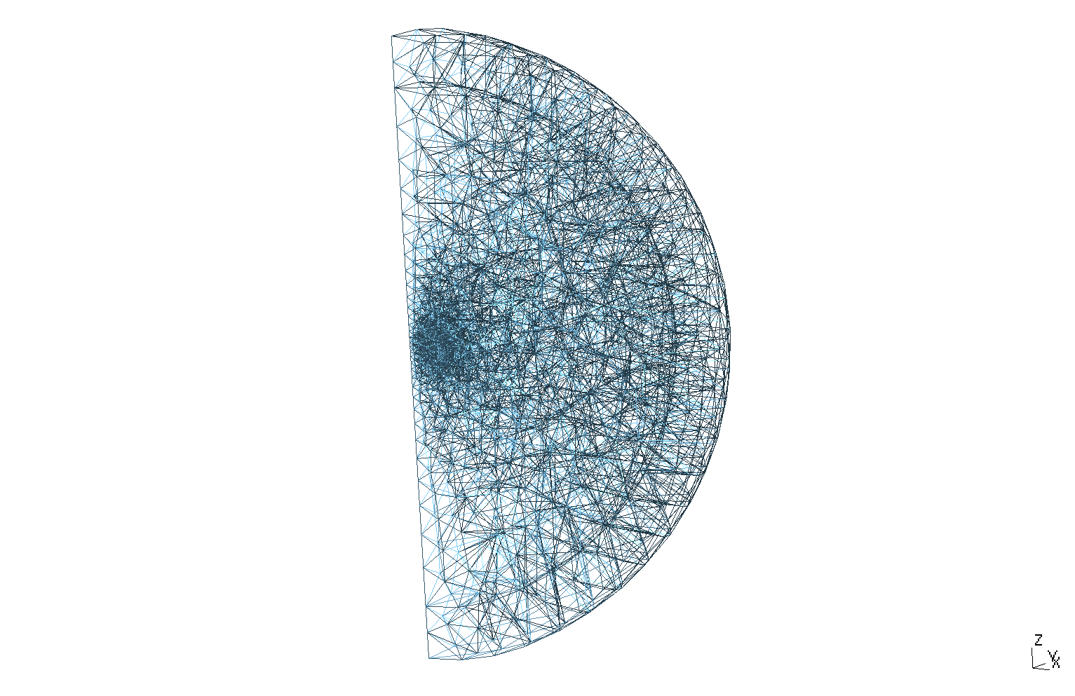
Mesh of Geometry

11. Results

11.1. Magnetic Potential Field

The magnetic potential field \(\mathbf{A}\) :

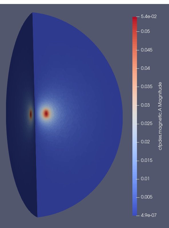
\(A (T.m)\)

The behavior of \(A\) on the \(O_r\) axis is as follows :

Table 1. L2 Error Norm for \(A\) on \(O_r\)
h	L2 Error Norm	L2 Relative Error Norm
\(1e-2\)	\(9.78512e-3\)	\(6.61\%\)
\(7e-3\)	\(8.03447e-3\)	\(5.43\%\)
\(5e-3\)	\(5.21347e-3\)	\(3.52\%\)
\(4e-3\)	\(4.96288e-3\)	\(3.36\%\)

11.2. Magnetic Field

The magnetic field \(\mathbf{B}\) is defined by :

\[ \mathbf{B} = \nabla \times \mathbf{A}\]

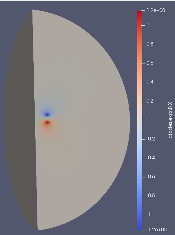
\(B_x (T)\) on Or axis

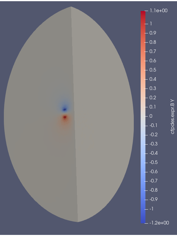
\(B_y (T)\) on Or axis

The behavior of \(\mathbf{B}_z\) on the \(O_z\) axis :

Table 2. L2 Error Norm for \(B_z\) on \(O_z\)
h	L2 Error Norm	L2 Relative Error Norm
\(1e-2\)	\(18.417352e-2\)	\(7.27\%\)
\(7e-3\)	\(8.989375e-2\)	\(3.55\%\)
\(5e-3\)	\(8.358335e-2\)	\(3.3\%\)
\(4e-3\)	\(5.451477e-2\)	\(2.15\%\)

12. References

Cecile Daversin - Catty. Reduced basis method applied to large non-linear multi-physics problems: application to high field magnets design. Electromagnetism. Université de Strasbourg, 2016. p56-64 PDF