Generate Comsol files with Python MPH
Python MPH is a Python library that allow the user to create or modify a Comsol file with Python. It uses the Java bridge provided by JPype to access the Comsol API and wraps it in a layer of python classes and functions. This library is developed by John Hennig, Max Elfner and Jacob Feder and it’s not officially related to Comsol. Hence, it is sometimes difficult to find the informations and specific functions that we need for different uses. But the python interface allows a large set of possibilities and is easier to use than the Java code of the Comsol files.
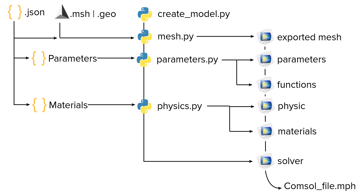
The utilization of Python MPH in this section is an introduction to a code that aims to be a generic bridge between .json files of Feelpp - CFPDE and .mph files that are used in the Comsol GUI. The goal is to take the different parts that compose the json file, translate and change them to create a new model which uses the CFPDE library of Comsol or even specific Physics templates depending on the formulation.
|
1. Data Files
The data files for the python code are available in Github here :
-
create_model.py - Edit the file
-
mesh.py - Edit the file
-
parameters.py - Edit the file
-
physics.py - Edit the file
2. Parameters for create_model.py
The different parameters that are needed to create the model on Comsol are :
-
folder : the folder where is situated the json file
-
file : the name of the json file
-
formulation : the physic that will be used (for now the option are hform and cfpde)
-
axis : is the model in axisymmetric coordinates ?
-
nonlin : is the model non linear ?
-
timedep : is the model time dependent ?
-
solveit : the program will solve the model in Comsol
-
openit : the program will open the model with comsol
import argparse
parser = argparse.ArgumentParser()
parser.add_argument("--folder", help="give folder of json file", type=str, default="../cylinder")
parser.add_argument("--file", help="give json file", type=str, default="cylinder.json")
parser.add_argument("--formulation", help="give formulation", type=str, default="hform")
parser.add_argument("--axis", help="is the model in axisymmetric coord", action='store_true')
parser.add_argument("--nonlin", help="is the model non linear", action='store_true')
parser.add_argument("--timedep", help="is the model timedep", action='store_true')
parser.add_argument("--solveit", help="solve the model ?", action='store_true')
parser.add_argument("--openit", help="open with comsol ?", action='store_true')
args = parser.parse_args()
3. Loading the mesh
Once the json is loaded, the program will load the mesh given in the "Meshes" part of the json into the mph file for Comsol. But as Comsol only accept mesh in .nas or .bdf format, the program first need to convert the .geo or .msh of the json using the Gmsh API.
def meshing_nastran(data, folder) :

    # Loading the geometry or mesh given by the json
    meshfilename=re.search('\$cfgdir\/(.*)', data["Meshes"]["cfpdes"]["Import"]["filename"]).group(1)
    if folder.endswith("/") :
        gmsh.open(folder+meshfilename)
    else :
        gmsh.open(folder+"/"+meshfilename)


    if meshfilename.endswith(".geo") :                          # if geometry is .geo
        gmsh.model.mesh.generate(2)                             # generating mesh
        bdffilename=meshfilename.removesuffix(".geo")+".bdf"
        gmsh.write(bdffilename)                                 # exporting in .bdf
    elif meshfilename.endswith(".msh") :                        # if geometry is .msh
        bdffilename=meshfilename.removesuffix(".msh")+".bdf"
        gmsh.write(bdffilename)                                 # exporting in .bdf

    gmsh.clear()

    return meshfilename, bdffilename
After that we are able to import the mesh into the .mph file :
def import_mesh(model, bdffilename, axis=0) :
    ### Create empty geometry for the imported mesh
    print("Info    : Creating Geometry...")
    geometries = model/'geometries'
    geometry = geometries.create(2, name='geometry')
    if axis :
        geometry.java.axisymmetric(True) # axisymmetric model
    print("Info    : Done creating Geometry")

    ### Importing the mesh from a .nas file
    print("Info    : Importing Mesh...")
    meshes = model/'meshes'
    mesh1 = meshes.create(geometry, name='mesh1')
    imported=mesh1.create("Import")
    imported.property('source', 'nastran')
    imported.property('data', 'mesh')
    imported.property('facepartition', 'minimal')
    imported.property('filename', bdffilename)
    model.mesh() # Build the mesh in order to select its parts later
    print("Info    : Done importing Mesh")
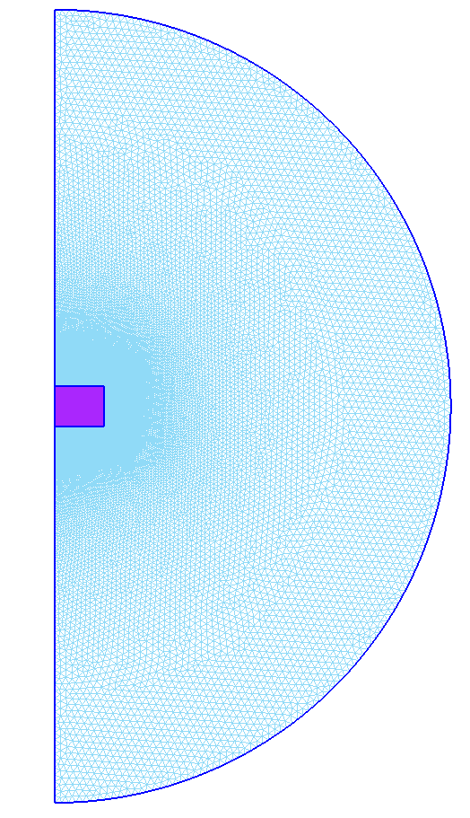
Mesh in GMSH
|
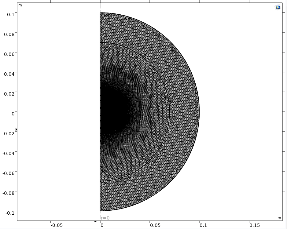
Mesh imported in Comsol
|
Finally, once the mesh is imported, we need to retrieve the physical names of our mesh, because Comsol assigns a random number to each one of them, which are not easyly usable with python mph. So we create a "Selection" for each physical names that will contain the numbers of the physical object that are in it :
def creating_selection(model, meshfilename, folder) :
    if folder.endswith("/") :
        gmsh.open(folder+meshfilename)
    else :
        gmsh.open(folder+"/"+meshfilename)

    # Checking if two physical groups have the same ID
    print("Info    : Checking Selections")
    selections = model/'selections'
    check_selection = [child.name() for child in selections.children()]
    if len(check_selection) != len(np.unique(check_selection)) :
        print("ERROR   : Some physical lines and physical surface have the same ID")
        exit(1)
    print("Info    : Done checking Selections\n             --> Selections are valid")

    # Assigning the domain numbers of Comsol to the physical groups' names
    print("Info    : Creating Selection's dictionnary...")
    selection_import={}
    groups = gmsh.model.getPhysicalGroups()
    for g in groups :
        dim = g[0]
        tag = g[1]

        name = gmsh.model.getPhysicalName(dim, tag)
        ent = gmsh.model.getEntitiesForPhysicalGroup(dim,tag)
        tab = []
        for child in selections.children():
            for i in ent :
                if " "+str(i)+" " in child.name() and child.selection()[0] not in tab:
                    tab.append(child.selection()[0])
        selection_import[name]=tab

    print("Info    : Done creating Selection's dictionnary")
    # print(selection_import)
    gmsh.clear()
    # selection_import = import_mesh(model,data,axisymmetric)

    return selection_import
4. Importing the parameters and functions
Once the mesh is loaded, we can translate the parameters and functions of the json file into parameters in Comsol :
### Create parameters
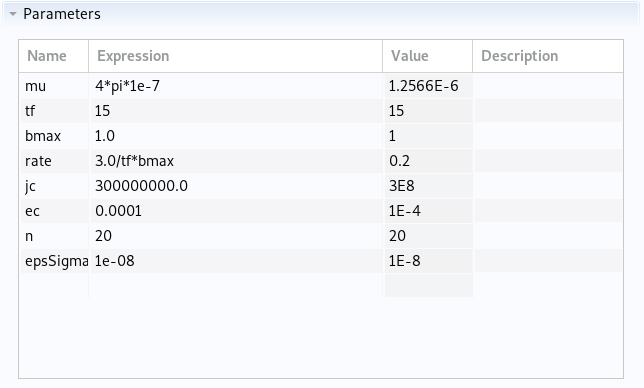
def parameters_and_functions(model, data) :
parameters = model/'parameters'
functions = model/'functions'
# (parameters/'Parameters 1').rename('parameters')
if "Parameters" in data : # export parameters from json if there is a section parameters
print("Info : Loading Parameters...")
param = data["Parameters"]
for p in param :
if type(param[p])==str :
if re.search("(<|>|<=|>=|==|!=)", param[p]) : # if the parameter is a function, creating a function
func = functions.create('Analytic', name=p)
func.property('funcname', p)
func.property('args', 't')
func.property('expr', param[p].split(":")[0])
func.property('plotargs', [['t', '0', 'tf']])
else :
model.parameter(p,param[p].split(":")[0]) # if the parameter is a str, keeping ononliny the expression part
else :
model.parameter(p,str(param[p]))
print("Info : Done loading Parameters")
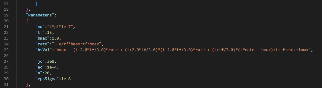
Parameters in cylinder.json
|
Parameters imported in Comsol
|
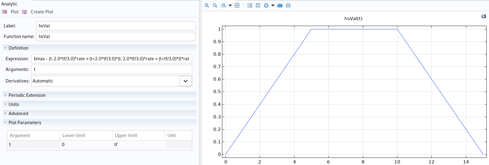
Function imported in Comsol
|
5. Creating the physic
The physic is the biggest part of the program. The goal is to use one of the physic library of Comsol and adapt the model in the json file to it. The most obvious choice is the physic CFPDEs in Comsol, with which we can easily translate the Feelpp language in the json file, but it is sometime easier to use other physics that are harder to translate here, but which gives better performance on Comsol. For now, only the CFPDEs library and the Magnetic Field Formulation library (corresponding to the H-Formulation) are implemented.
5.1. Magnetic Field Formulation
First the function create the physic mfh for Magnetic Field Formulation :
def physic_and_mat(model, data, selection_import, formulation, axis=0, non_linear=0) :

    physics = model/'physics'
    materials = model/'materials'
    geometry = (model/'geometries').children()[0]
    equations = data["Models"]["cfpdes"]["equations"]
    functions = model/'functions'

    ### Create the physic and materials
    print("Info    : Creating Physics and Materials...")
    if formulation == 'hform' :
        mfh = physics.create('MagneticFieldFormulation', geometry, name='Magnetic Field Formulation')
        mfh.java.prop("DivergenceConstraint").set("DivergenceConstraint", False)  # Disabling the Divergence Cosntraint (not used here)
        (mfh/'Faraday\'s Law 1').property('ConstitutiveRelationJcE', 'ElectricalResistivity')
        index=1
Physic of conductor in Comsol
|
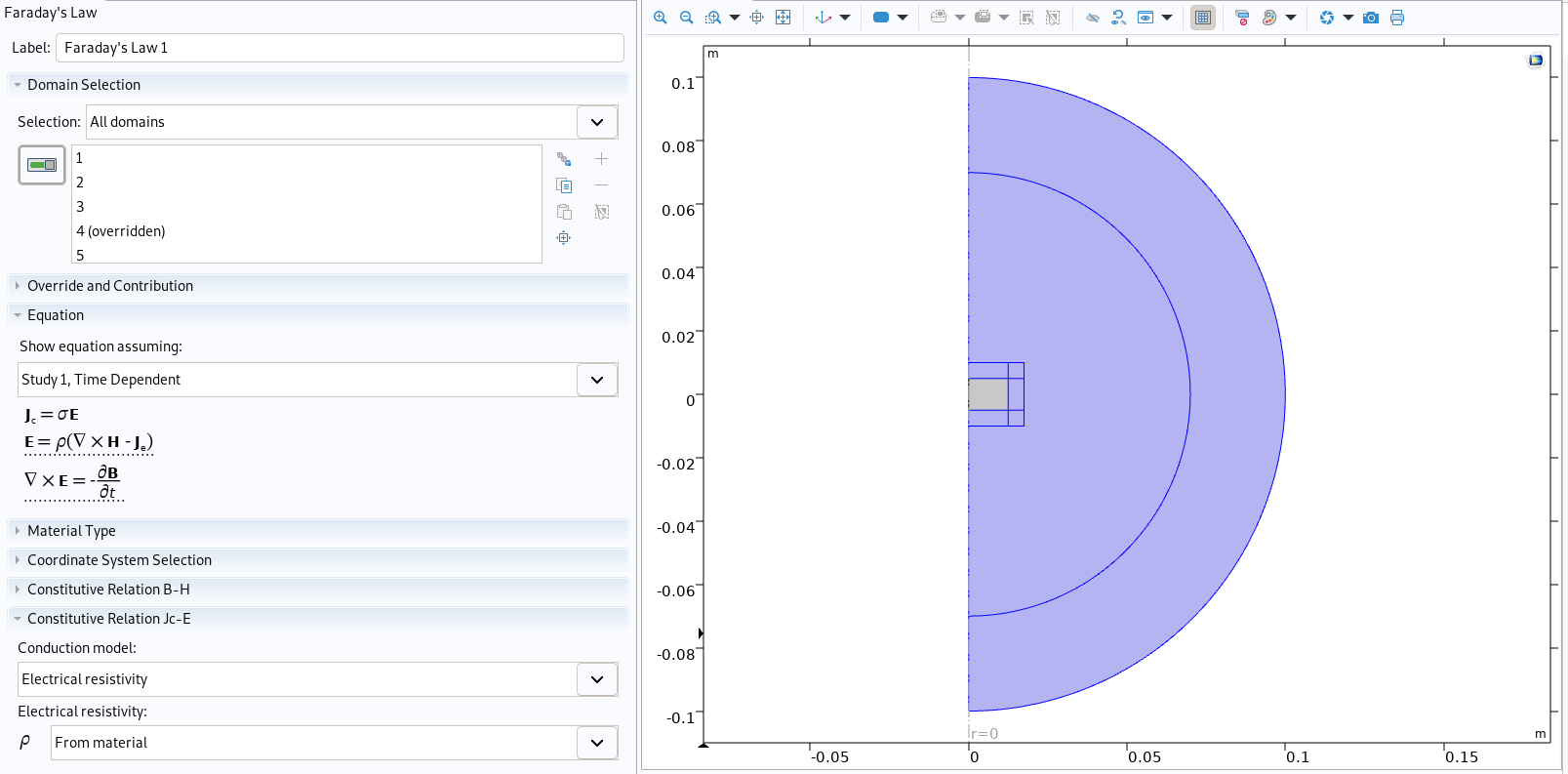
Physic of air in Comsol
|
Then, each material is created and filled depending on its name. This will also add the E-J power law in the conductor material as this program is made to recreate models of superconductors :
for mat in mater : # for each materials in the json, creating the law and material in comsol
print("Info : Creating physic for material \"" + mat +"\"..." )
if "markers" in mater[mat] :
markers=mater[mat]["markers"]
else :
markers = mat # if there is no markers the material is defined by the title
if type(markers) == str :
markers=[markers]
if mat == "Air" :
air1 = materials.create('Common', name='Air 1')
air1.select(np.concatenate([selection_import[markers[i]] for i in range(len(markers))]))
air1.java.propertyGroup('def').set('relpermittivity','1')
air1.java.propertyGroup('def').set('relpermeability','1')
if "rho_air" in mater[mat] :
rho_air = mater[mat]["rho_air"]
else :
rho_air = 1e2 # rho_air is usually not defined, this is a default value
air1.java.propertyGroup('def').set('resistivity',str(rho_air))
else :
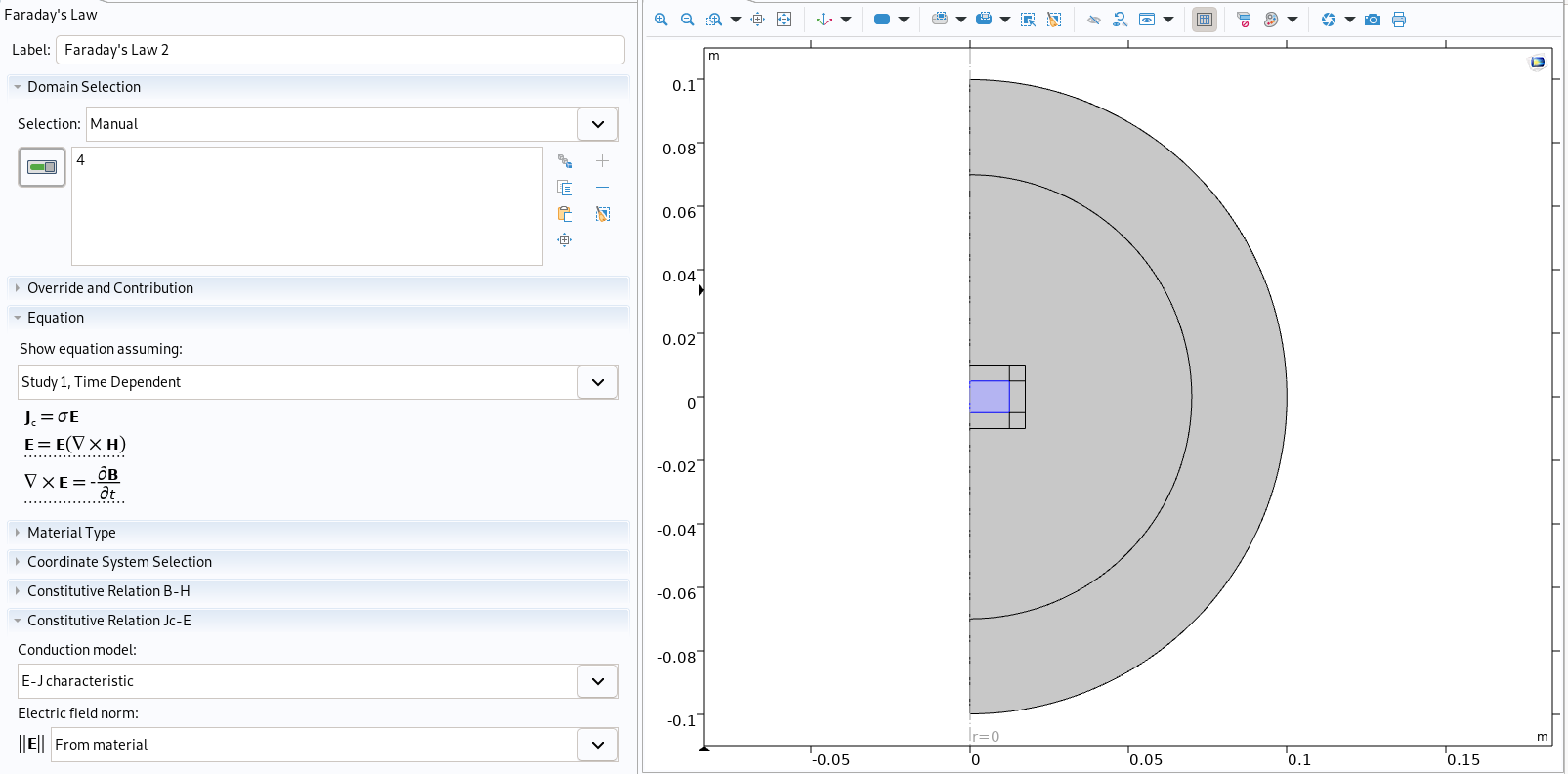
fl = mfh.create('FaradaysLaw',2, name='Faraday\'s Law 2')
fl.select(np.concatenate([selection_import[markers[i]] for i in range(len(markers))]))
if non_linear :
fl.property('ConstitutiveRelationJcE', 'EJCharacteristic')
else :
fl.property('ConstitutiveRelationJcE', 'ElectricalResistivity')
fl.property('materialType', 'solid')
cond = materials.create('Common', name='Conductor'+str(index))
cond.select(np.concatenate([selection_import[markers[i]] for i in range(len(markers))]))
if non_linear :
cond.java.propertyGroup().create("EJCurve", "E-J_characteristic")
cond.java.propertyGroup('EJCurve').set('normE', mater[mat]["normE"].split(":")[0])
else :
cond.java.propertyGroup('def').set('resistivity','1/(sigma_'+mat+')')
cond.java.propertyGroup('def').set('relpermittivity','1')
cond.java.propertyGroup('def').set('relpermeability','1')
index=index+1
print("Info : Done creating physic for material \"" + mat +"\"" )
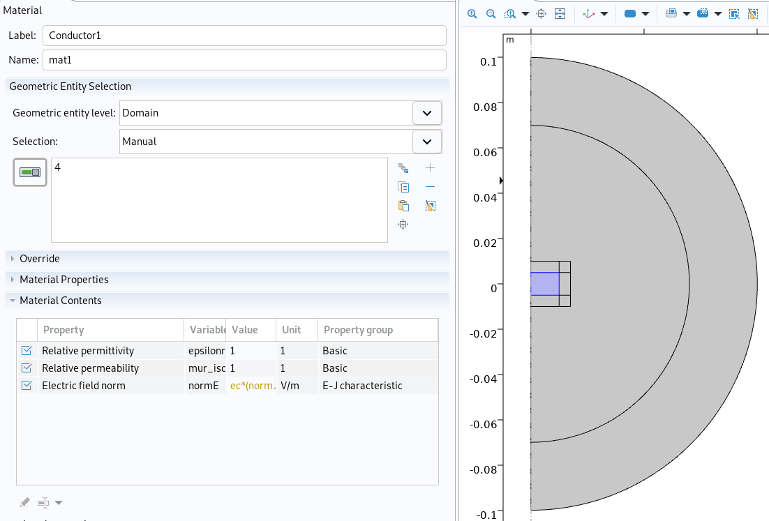
Conductor material in Comsol
|
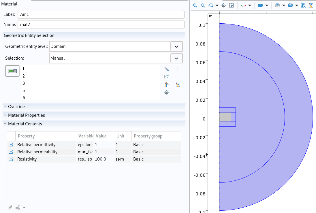
Air material in Comsol
|
Finally the boundary conditions are implemented, here in the form of an applied magnetic field :
        # loading boundary conditions (only dirichlet for now)
        print("Info    : Creating Boundary Conditions..." )
        index=1
        for i in range(len(equations)) :
            Bc = data["BoundaryConditions"][equations[i]["name"]]["Dirichlet"]

            for b in Bc :

                if "markers" in Bc[b] :
                    markers=Bc[b]["markers"]
                else :
                    markers = b

                if type(markers) == str :
                    markers=[markers]

                expr = Bc[b]["expr"]
                if type(expr) == str :
                    expr = expr.split(":")[0]  # keeping only the expression part
                    for child in functions.children() :
                        if child.name() in expr :  # if the boundary condition contains a function
                            # expr=expr.replace(child.name(),child.name()+"("+child.property('args')[0]+")")
                            expr = child.name()+"("+child.property('args')[0]+")"  # adding (arg) next to the function
                else :
                    expr = str(expr)

                mf = mfh.create('MagneticFieldBoundary',1, name='Magnetic Field '+str(index))
                mf.select(np.concatenate([selection_import[markers[i]] for i in range(len(markers))]))
                mf.property('H0', ['0', '0', expr + "/mu" ])
                index=index+1
        print("Info    : Done creating Boundary Conditions" )
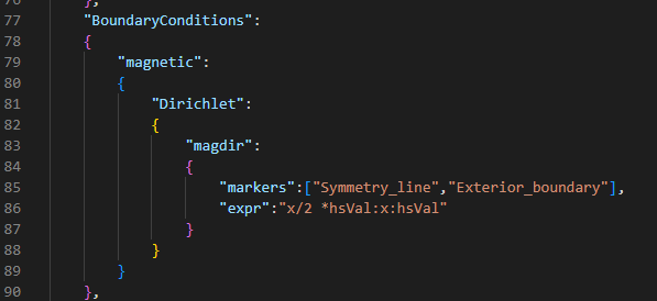
Boundary condition in cylinder.json
|
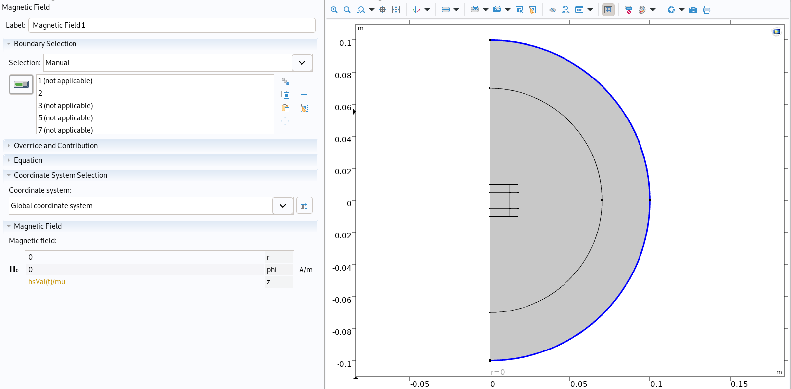
Boundary condition imported in Comsol
|
5.2. CFPDEs
The program creates the physic cfpdes, detects different coefficient for each material and import them on Comsol :
def physic_and_mat(model, data, selection_import, formulation, axis=0, non_linear=0) :

    physics = model/'physics'
    materials = model/'materials'
    geometry = (model/'geometries').children()[0]
    equations = data["Models"]["cfpdes"]["equations"]
    functions = model/'functions'

    ### Create the physic and materials
    print("Info    : Creating Physics and Materials...")
    #[...]

    elif formulation == 'cfpdes' :
        letters = {'c':'c', 'beta':'be', 'a':'a', 'alpha':'al', 'f':'f', 'gamma':'ga', 'd':'da'}

        for eq in range(len(equations)) :
            cfpde = physics.create('CoefficientFormPDE', geometry, name='Coefficient Form PDE '+equations[eq]["name"])
            mater = data["Materials"]
            for mat in mater :  # for each materials in the json, creating the law and material in comsol

                print("Info    : Creating physic for material \"" + mat +"\"..." )
                if "markers" in mater[mat] :
                    markers=mater[mat]["markers"]
                else :
                    markers = mat  # if there is no markers the material is defined by the title

                if type(markers) == str :
                    markers=[markers]

                if mat == "Air" :
                    cf = cfpde/'Coefficient Form PDE 1'
                    cf.property('f', '0')
                    cf.property('c', '0')
                    cf.property('da', '0')
                    for p in mater[mat]:
                        # for i in range(len(equations)) :
                            if p.startswith(equations[eq]["name"]) :
                                l=p.removeprefix(equations[eq]["name"]+'_')
                                if type(mater[mat][p]) == str :
                                    expr = mater[mat][p].split(":")[0]
                                else :
                                    expr = str(mater[mat][p])

                                if re.search('{(.*)}', expr) :
                                    expr = re.search('{(.*)}', expr).group(1)
                                    expr = expr.split(",")
                                    if axis :
                                        for i in range(len(expr)) :
                                            expr[i] = expr[i].replace('x','r')+'/r'
                                else :
                                    if axis :
                                        expr = expr.replace('x','r')+'/r'

                                cf.property(letters[l], expr)
                else :
                    cf = cfpde.create('CoefficientFormPDE',2, name='CFPDE '+mat)
                    cf.select(np.concatenate([selection_import[markers[i]] for i in range(len(markers))]))
                    cf.property('f', '0')
                    cf.property('c', '0')
                    cf.property('da', '0')
                    for p in mater[mat]:
                        # for i in range(len(equations)) :
                            if p.startswith(equations[eq]["name"]) :
                                l=p.removeprefix(equations[eq]["name"]+'_')
                                if type(mater[mat][p]) == str :
                                    expr = mater[mat][p].split(":")[0]
                                    for child in functions.children() :
                                        if child.name() in expr :  # if the boundary condition contains a function
                                            expr=expr.replace(child.name(),child.name()+"("+child.property('args')[0]+")")
                                else :
                                    expr = str(mater[mat][p])

                                if re.search('{(.*)}', expr) :
                                    expr = re.search('{(.*)}', expr).group(1)
                                    expr = expr.split(",")
                                    if axis :
                                        for i in range(len(expr)) :
                                            expr[i] = expr[i].replace('x','r')+'/r'
                                else :
                                    if axis :
                                        expr = expr.replace('x','r')+'/r'


                                cf.property(letters[l], expr)
                print("Info    : Done creating physic for material \"" + mat +"\"" )
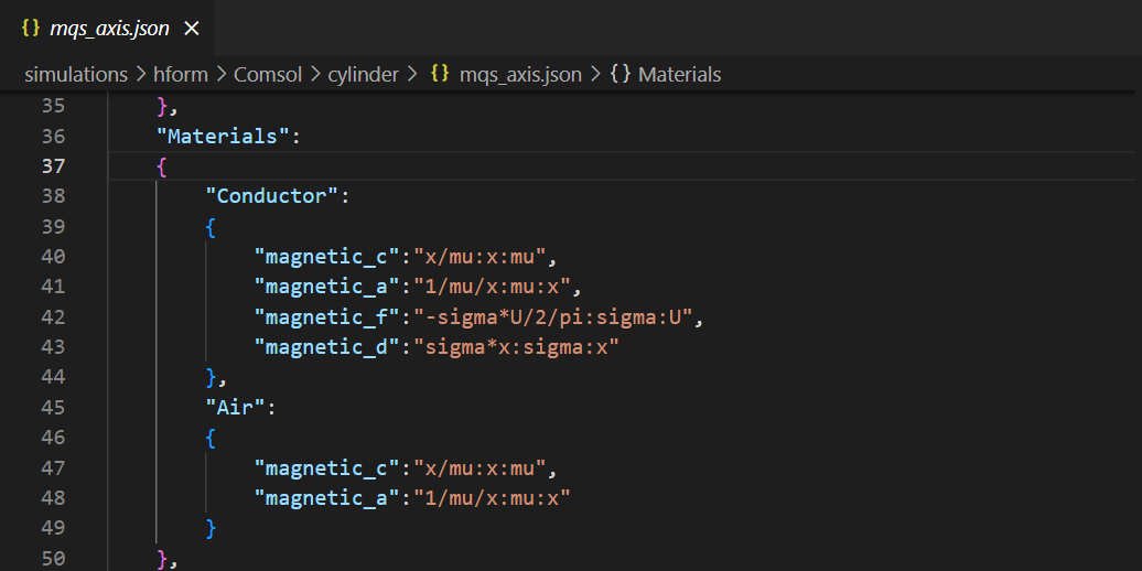
Materials on mqs_axis.json
|
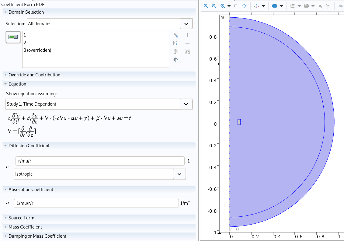
Physic of air in Comsol
|
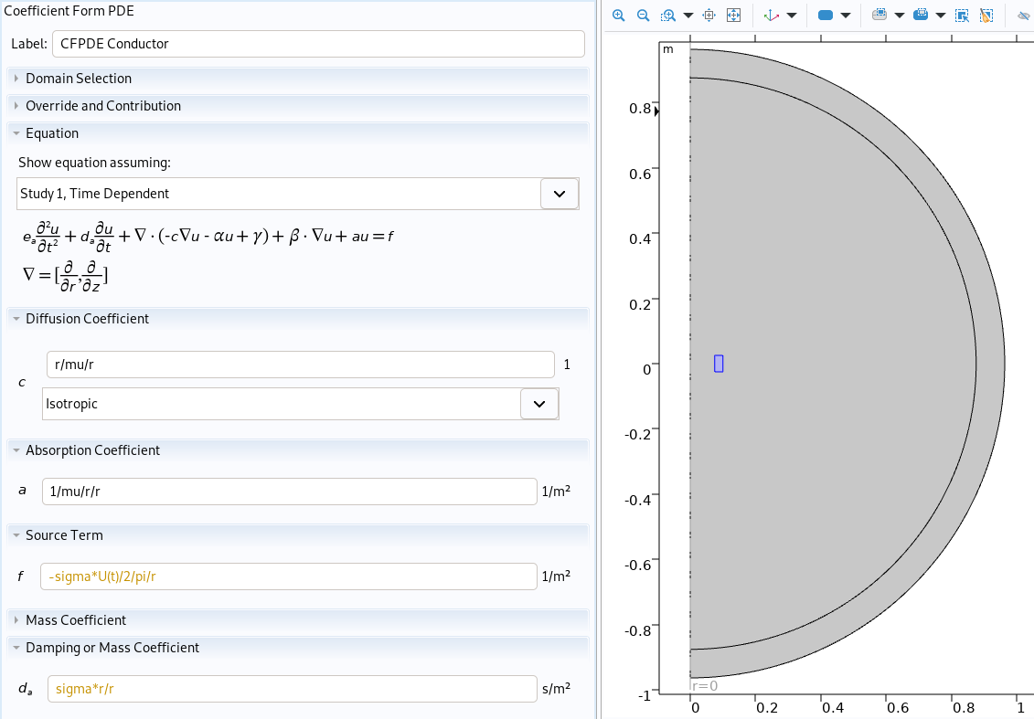
Physic of conductor in Comsol
|
The Dirichlet boundary conditions are also implemented :
    # loading boundary conditions (only dirichlet for now)
    print("Info    : Creating Boundary Conditions..." )
    index=1
    # for i in range(len(equations)) :
    if 'Dirichlet' in data["BoundaryConditions"][equations[eq]["name"]] :
        Bc = data["BoundaryConditions"][equations[eq]["name"]]["Dirichlet"]

        for b in Bc :

            if "markers" in Bc[b] :
                markers=Bc[b]["markers"]
            else :
                markers = b

            if type(markers) == str :
                markers=[markers]

            expr = Bc[b]["expr"]
            if type(expr) == str :
                expr = expr.split(":")[0]  # keeping only the expression part
                for child in functions.children() :
                    if child.name() in expr :  # if the boundary condition contains a function
                        # expr=expr.replace(child.name(),child.name()+"("+child.property('args')[0]+")")
                        expr = child.name()+"("+child.property('args')[0]+")"  # adding (arg) next to the function
            else :
                expr = str(expr)

            dir = cfpde.create('DirichletBoundary',1, name='Dirichlet Boundary Condition  '+str(index))
            dir.select(np.concatenate([selection_import[markers[i]] for i in range(len(markers))]))
            dir.property('r', expr)
            index=index+1
    print("Info    : Done creating Boundary Conditions" )

print("Info    : Done creating Physics and Materials")
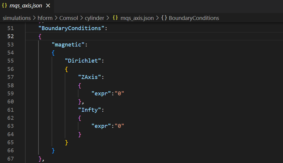
Boundary condition in mqs_axis.json
|
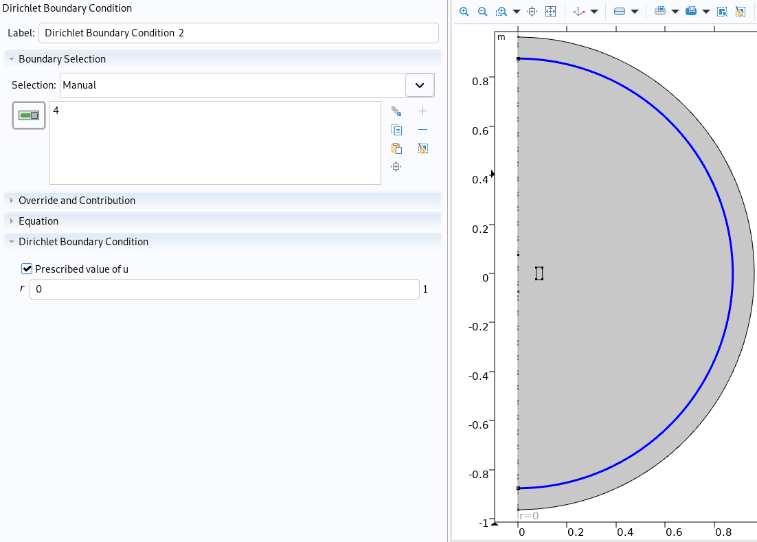
Boundary condition imported in Comsol
|
6. Creating the solver
The solver can be created to be time-dependent :
### Create time dependent solver
studies = model/'studies'
solutions = model/'solutions'
batches = model/'batches'
study = studies.create(name='Study 1')

if args.timedep :
    print("Info    : Creating Time-Dependent Solver..." )
    step = study.create('Transient', name='Time Dependent')
    step.property('tlist','range(0,0.1,tf)')
    solution = solutions.create(name='Solution 1')
    solution.java.study(study.tag())
    solution.java.attach(study.tag())
    solution.create('StudyStep', name='equations')
    solution.create('Variables', name='variables')
    solver = solution.create('Time', name='Time-Dependent Solver')
    solver.property('tlist', 'range(0, 0.1, tf)')

    print("Info    : Done creating Time-Dependent Solver..." )
And it can be created to be static :
else :
    print("Info    : Creating Stationary Solver..." )
    step = study.create('Stationary', name='Stationary')
    solution = solutions.create(name='Solution 1')
    solution.java.study(study.tag())
    solution.java.attach(study.tag())
    solution.create('StudyStep', name='equations')
    solution.create('Variables', name='variables')
    solver = solution.create('Stationary', name='Stationary Solver')

    print("Info    : Done creating Stationary Solver..." )
There are also some small adjustements if the problem is non-linear. In this case we had :
    if args.nonlin :
        ## Special changes for non-linear models
        fcoupled = solver/'Fully Coupled'
        fcoupled.property('jtech', 'once')
        fcoupled.property('maxiter', '25')
        fcoupled.property('ntolfact', '0.1')
7. References
-
[Python MPH] mph.readthedocs.io/en/stable/index.html