The adaptative VSVO Method
This section will present an algorithm created to adapt both the order and the time step to efficiently and more precisely solve EDPs using a backward Euler FEM code. This algorithm is presented by V. P. DeCaria in the dissertation Variable Stepsize, Variable Order Methods for Partial Differential Equations.
1. Algorithm Variable Stepsize, variable Order 1 and 2
First, let’s give the method for the initial problem :
We write \(\Delta t_n\) as the \(n^{th}\) time stepsize. We have also \(t^{n+1}=t^n + \Delta t_n\) and \(y^n\) an approximation for \(y(t_n)\). \(TOL\) is the tolerance chosen by the user on the allowable error by step.
1.1. Step 1 : Backward Euler
1.1.1. Implementation in FreeFEM
We start a While that will stop when the current time \(T\) reaches the final time \(T\) :
while (t<=T){

     // previous solution are saved in case of
     // returning to previous time step
     ysave = yppp;
     yppp = ypp;
     ypp = uold;
     uold = u; //equivalent to u^{n-1} = u^n

     // STEP 1 : backward euler
     // Solve
     mqs;
1.2. Step 2 : Time Filter
with \(\omega_n=\frac{\Delta t_n}{\Delta t_{n-1}}\) the filtering weight.
1.3. Step 3: Estimate Error in \(y_{(1)}^{n+1}\) and \(y_{(2)}^{n+1}\)
We compute an estimation of the local errors in this step. \(Est_1\) provides an estimation of the local error of the first order approximation and \(Est_2\) of the second order approximation.
1.3.1. Implementation in FreeFEM
while (t<=T){
    //[...]

    // STEP 3 : estimate error
     est1=y2-y1;
     est2=wp*wn*(1+wn)/(1+2*wn+wp*(1+4*wn+3*wn^2))*(
               y2
          -(1+wn)*(1+wp*(1+wn))/(1+wp)*uold
          +wn*(1-wp*(1+wn))*ypp
          -wp^2*wn*(1+wn)/(1+wp)*yppp
          );

     est1l2 = sqrt( int2d(Th)((est1)^2));
     est2l2 = sqrt( int2d(Th)((est2)^2));

    // safety net in order to not divide by 0 later
     if (est1l2==0) est1l2=1e-20;
     if (est2l2==0) est2l2=1e-20;
1.4. Step 4: Check if tolerance is satisfied
If \(||EST_1||<TOL\) or \(||EST_2||<TOL\), at least one approximation is correct, got to Step 5a. Otherwise the step is rejected, got to Step 5b
1.5. Step 5a: At least one approximation satisfy TOL
If both approximation are acceptable, set
And set
(The approximation which have the largest estimated \(\Delta t\) is chosen to advance the solution.)
If only \(y^{(1)}\) (resp. \(y^{(2)}\)) satisfies \(TOL\), set \(\Delta t_{n+1}=\Delta t^{(1)}\) (resp. \(\Delta t^{(2)}\)), and \(y^{n+1}=y^{n+1}_(1)\) (resp. \(y^{n+1}=y^{n+1}_(2)\)). Proceed to Step 1 to calculate \(y^{n+2}\).
1.5.1. Implementation in FreeFEM
while (t<=T){
    //[...]

    else if (( est1l2 <= tol ) || (est2l2 <= tol)){
          // STEP 5a : At least one approx is accepted

          dt1 = 0.9*dt*sqrt(tol/est1l2);
          dt2 = 0.9*dt*(tol/est2l2)^(1/3.);

          dtpp = dtp;
          dtp = dt;
          if (( est1l2 <= tol ) && (est2l2 <= tol)){
               dt = max(dt1, dt2);
          }
          else if( est1l2 <= tol ){
               dt = dt1;
          }
          else{
               dt = dt2;
          }

          if (dt == dt1){
               u = y1;
          }
          else{
               u = y2;
          }
          tp = t;

          t = t + dt;
     }
1.6. Step 5b: Neither Approximation satisfy TOL
Set
Set
Return to Step 1 and try again.
1.6.1. Implementation in FreeFEM
while (t<=T){
    //[...]

    if (( est1l2 > tol ) && (est2l2 > tol)){
        // STEP 5b : Neither approximation satisfy TOL

        dtsave = dtpp;
        dtpp = dtp;
        dtp = dt;

        dt1 = 0.7*dt*sqrt(tol/est1l2);
        dt2 = 0.7*dt*(tol/est2l2)^(1/3.);

        dt = max(dt1, dt2);

        t = tp+dt;

        dtp = dtpp;
        dtpp = dtsave;

        u = uold;
        uold = ypp;
        ypp = yppp;
        yppp = ysave;
    }
    //[...]
}
1.7. Additionnal Implementations
This was the basic implementation of the VSVO Algorithm, but there are several standard features that are missing.
1.7.1. Maximum stepsize
We impose a maximum time step in order to have reasonable stepsize and to prevent at a certain level to go to the Step 5b because the timestep was really large. This feature appears only in the Step 5a as this is the step where the stepsize can increase.
real dtmax=1;

while (t<=T){
    //[...]

    else if (( est1l2 <= tol ) || (est2l2 <= tol)){
          // STEP 5a : At least one approx is accepted

          dt1 = 0.9*dt*sqrt(tol/est1l2);
          dt2 = 0.9*dt*(tol/est2l2)^(1/3.);

          dtpp = dtp;
          dtp = dt;
          if (( est1l2 <= tol ) && (est2l2 <= tol)){
               dt = max(dt1, dt2);
          }
          else if( est1l2 <= tol ){
               dt = dt1;
          }
          else{
               dt = dt2;
          }

          if (dt == dt1){
               u = y1;
          }
          else{
               u = y2;
          }
          // Check if dt>dtmax before t is changed
          if (dt>dtmax) dt=dtmax;

          tp = t;

          t = t + dt;
     }
1.7.2. Minimum stepsize
We impose a minimum time step in order to avoid the algorithm to be too long. If the timestep is always decreasing and the estimation is not acceptable each time, then it’s a reasonable choice to go to the next time and start the process once again. This feature appears only in the Step 5b as this is the step where the stepsize can decrease.
real dtmax=1;

while (t<=T){
    //[...]

    if (( est1l2 > tol ) && (est2l2 > tol)){
          // STEP 5b : Neither approximation satisfy TOL

          dtsave = dtpp;
          dtpp = dtp;
          dtp = dt;

          dt1 = 0.7*dt*sqrt(tol/est1l2);
          dt2 = 0.7*dt*(tol/est2l2)^(1/3.);

          dt = max(dt1, dt2);

          // if dt<dtmin force it
          if (dt<dtmin){
               dt=dtmin;

               tp = t;

               t = t + dt;

          }
          // else try again last t with new dt
          else {
               t = tp+dt;

               dtp = dtpp;
               dtpp = dtsave;

               u = uold;
               uold = ypp;
               ypp = yppp;
               yppp = ysave;
          }
     }
1.7.3. Forced timestep
As the stepsize is variable, we cannot be sure that \(t\) will stop at certain values that we are interested in. That’s why being able to force \(t\) to go trough specific values is a must-have in this type of algorithm.
In order to do that, we creat a list with all the values we want \(t\) to go trought. Then before updating the new \(t\) in Step 5a and Step 5b, we check if the current \(t\) is in the list and if it is we go to the next one. Finally after applying the stepsize to obtain a new timestep, we check if the new timestep is not higher than the current value in the list and in this case we adapt the stepsize to reach precisely the forced value.
int nforced=3; //number of forced values
real[int] forcedtime = [1,20,22]
int force = 0; //index of forced values

while (t<=T){
     //[...]

     // STEP 4 : Check Tol
     if (( est1l2 > tol ) && (est2l2 > tol)){
          // STEP 5b : Neither approximation satisfy TOL

          //[...]

          // if dt<dtmin force it
          if (dt<dtmin){

               dt=dtmin;
               //check if t in forcedtime
               if (force<nforced) {
                    if (t==forcedtime[force]) force = force + 1;
               }

               tp = t;
               //check if t+dt!>forcedtime
               if (force<nforced) {
                    if ((t!=forcedtime[force]) && ((t+dt)>forcedtime[force])){
                         dt = forcedtime[force]-t;
                    }
               }

               t = t + dt;
          }
          // else try again last t with new dt
          else {
               //check if t+dt!>forcedtime
               if (force<nforced) {
                    if ((tp!=forcedtime[force]) && ((tp+dt)>forcedtime[force])){
                         dt = forcedtime[force]-tp;
                    }
               }

               t = tp+dt;

               //[...]
          }
     }
     else if (( est1l2 <= tol ) || (est2l2 <= tol)){
          // STEP 5a : At least one approx is accepted

          //check if t in forcedtime
          if (force<nforced) {
               if (t==forcedtime[force]) force = force + 1;
          }

          dt1 = 0.9*dt*sqrt(tol/est1l2);
          dt2 = 0.9*dt*(tol/est2l2)^(1/3.);

          dtpp = dtp;
          dtp = dt;
          if (( est1l2 <= tol ) && (est2l2 <= tol)){
               dt = max(dt1, dt2);
          }
          else if( est1l2 <= tol ){
               dt = dt1;
          }
          else{
               dt = dt2;
          }

          if (dt == dt1){
               u = y1;
          }
          else{
               u = y2;
          }

          tp = t;
          //check if t+dt!>forcedtime
          if (force<nforced) {
               if ((t!=forcedtime[force]) && ((t+dt)>forcedtime[force])){
                    dt = forcedtime[force]-t;
               }
          }

          t = t + dt;

     }

}
2. Implementation on an example
We will use this algorithm on a simple example of Maxwell Quasi Static problem, time-dependent with the A Formulation for a geometry of a torus surrounded by air in axisymmetric coordinates.
2.4. Results
Let’s compare the evolution of stepsize compared to the evolution of the electrical tension \(U\) as a function of time. The maximum stepsize is \(\Delta t_{max}=1\) :
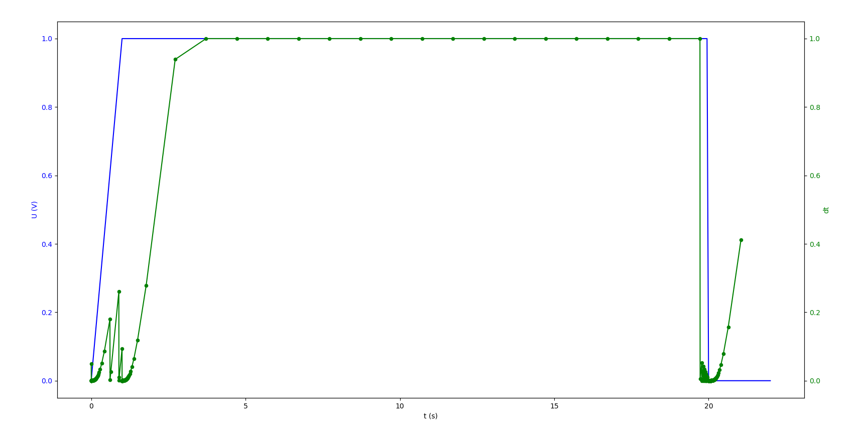
Time evolution of the variable stepsize compared to the electric tension
|
We can observe that when the tension is constant, the stepsize goes quickly to the maximum stepsize, but when \(U\) undergoes important changes, the stepsize becomes very small to be more precise at those times.
We also can see that, when compared to the analytic solution, the model using the VSVO Algorithm is more precise than the model with constant stepsize :
No VSVO |
VSVO |
L2 relative error Norm : \(1.72 \%\) |
L2 relative error Norm : \(0.66 \%\) |