Test Case : FreeFEM - Bulk Cylinder in Axisymmetric coordinates

1. Introduction

This is the test case of High-Temperature Superconductors with the A-V Formulation and Gauge Condition on a cylinder geometry surrounded by air in axisymmetric coordinates. The formulation used here is the Formulation in axisymmetric coordinates.

2. Run the Calculation

The command line to run this case is :

    ff-mpirun -np 4 mqs.edp -wg

3. Data Files

The case data files are available in Github here :

EDP file - Edit the file

4. Equation

The A-V Formulation in axisymmetric coordinates is :

A Formulation in axisymmetric coordinates

\[ -\frac{1}{\mu}\Delta A_\theta + \frac{1}{\mu r^2}A_\theta + \sigma \frac{\partial A_\theta}{\partial t} =0 \quad\text{on } \Omega^{axis} \quad \text{(A Axis)}\]

With :

\(A_{\theta}\) : \(\theta\) component of potential magnetic field
\(\sigma\) : electric conductivity \(S/m\) described by the e-j power law : \(\sigma=\frac{J_c}{E_c}\left(\frac{\mid\mid e\mid\mid}{E_c}\right)^{(1-n)/n} = \frac{J_c}{E_c}\left(\frac{\mid\mid -\partial_t A_\theta\mid\mid}{E_c}\right)^{(1-n)/n}\)
\(\mu\) : electric permeability \(kg/A^2/S^2\)

5. Geometry

The geometry is a rectangle in axisymmetric coordinates \((r,z)\) representing a bulk cylinder, surrounded by air.

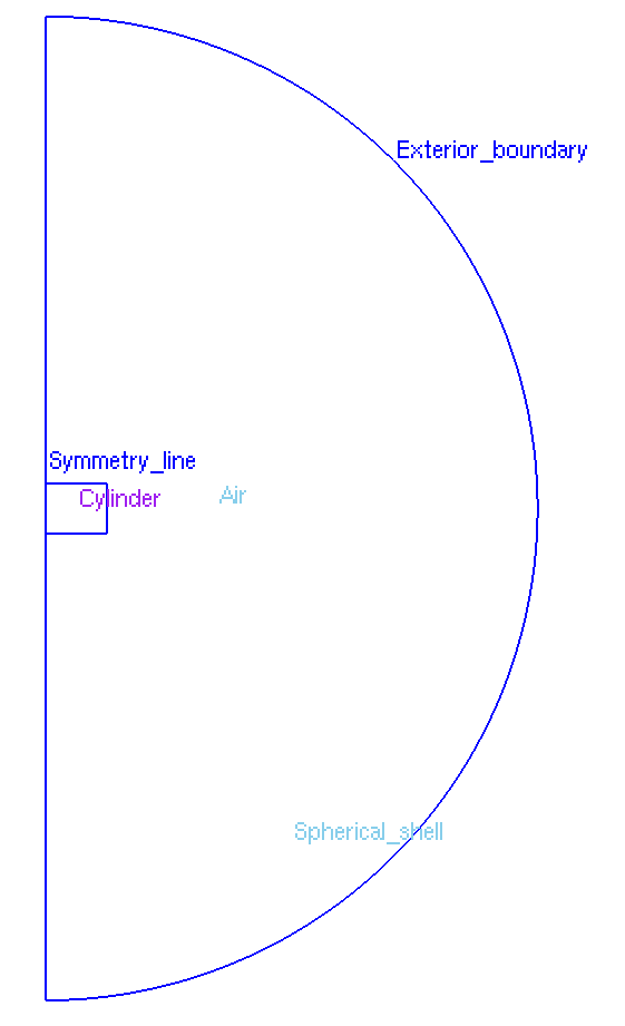
Geometry in Axisymmetrical cut

The geometrical domains are :

Cylinder : the cylinder, composed by a conductor
Air & Spherical Shell : the air surrounding Conductor
- Symmetry Line : Air 's bound, correspond to \(Oz\) axis (\(\{(z,r), \, z=0 \}\))
- Exterior Boundary : the rest of the Air 's bound

Symbol

Description

value

unit

\(R\)

radius of cylinder

\(0.00125\)

\(H_{cylinder}\)

height of cylinder

\(0.001\)

\(R_{inf}\)

radius of infty border

\(0.1\)

Geometry on EDP file

real BoxRadius = 0.1;			//"Infinite" boundary
real SupraRadius = 0.0125;
real SupraHeight = 0.01;

int BoxWall = 10;
int Axis1 = 11;
int Axis2 = 12;
int Axis3 = 13;

border b1(t=-pi/2, pi/2){x=BoxRadius*cos(t); y=BoxRadius*sin(t); label=BoxWall;};

int nnA = max(2., BoxRadius*nn/2.);
border axis1(t=0., 1.){x=0; y=-BoxRadius+(BoxRadius-SupraHeight/2.)*t; label=Axis1;};
border axis2(t=0., 1.){x=0; y=BoxRadius-(BoxRadius-SupraHeight/2.)*t; label=Axis2;};

border s1(t=0., 1.){x=(SupraRadius)*t; y=-SupraHeight/2.;};
border s2(t=0., 1.){x=SupraRadius; y=-SupraHeight/2.+SupraHeight*t;};
border s3(t=0., 1.){x=SupraRadius-(SupraRadius)*t; y=SupraHeight/2.;};
border s4(t=0., 1.){x=0; y=SupraHeight/2.-SupraHeight*t; label=Axis3;};

The mesh is also generated in FreeFEM :

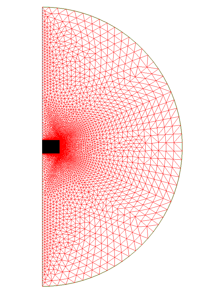
Mesh of Geometry

6. Parameters

The parameters of the problem are :

On Cylinder :

Symbol

Description

Value

Unit

\(\mu=\mu_0\)

magnetic permeability of vacuum

\(4\pi.10^{-7}\)

\(kg \, m / A^2 / S^2\)

\(t_f\)

final time

\(15\)

\(s\)

\(b_{max}\)

maximum applied field

\(1\)

\(T\)

\(rate\)

rate of the applied field raise

\(\frac{3}{tf}b_{max}\)

\(T/s\)

\(hsVal\)

time ramp for the applied field

\(\begin{cases}rate*t &\quad\text{if }t<\frac{t_f}{3}\\b_{max} &\quad\text{if }t<\frac{2t_f}{3}\\b_{max} - (t-\frac{2t_f}{3})*rate &\quad\text{if }t>\frac{2t_f}{3}\end{cases}\)

\(T\)

\(J_c\)

critical current density

\(3.10^8\)

\(A/m^2\)

\(E_c\)

threshold electric field

\(10^{-4}\)

\(V/m\)

\(n\)

material dependent exponent

\(20\)

\(\sigma\)

electrical conductivity (described by the \(e-j\) power law)

\(\frac{J_c}{E_c}\left(\frac{\mid\mid e\mid\mid}{E_c}\right)^{(1-n)/n}\)

\(S/m\)

On Air :

Symbol

Description

Value

Unit

\(\mu=\mu_0\)

magnetic permeability of vacuum

\(4\pi.10^{-7}\)

\(kg \, m / A^2 / S^2\)

On the EDP file, the parameters are written :

Parameters on EDP file

real Mu0 = 4.*pi*1.e-7;
func Nu = 1./Mu0;

real T = 15;
real dt = .05;
real t = 0;

real bmax = 1;
real rate = 3.0/T*bmax;

real jc = 3.e+8;
real ec = 1.e-4;
real epsSigma = 1.e-8;
int n = 20;

macro sigma(u) x*jc/ec*1.0/(epsSigma + ( abs(-(u-uold)/dt/ec )^((n-1.0)/n) ))

7. Weak Formulation

Weak formulation of A Formulation in two dimensions approximation

\[ \int_{\Omega_c^{axis}}{\sigma \frac{\partial A_\theta}{\partial t} \, \phi \ rdrdz } + \int_{\Omega^{axis}}{ \frac{1}{\mu} \nabla A_\theta \cdot \nabla \phi \ rdrdz }+\int_{\Omega^{axis}}{ \frac{1}{\mu r} A_\theta \cdot \phi \ drdz } = 0 \hspace{1cm} \text{(Weak A Axi)}\]

8. Implementation of Weak Formulation

On FreeFEM, we need to implement the weak the Weak Formulation :

On the EDP file, the weak formulation is written :

Weak Formulation on EDP file

    problem mqs(u, v, solver=sparsesolver, eps=1.e-10)
     = int2d(Th)(sigma(uu)*(region==Supra) * u'*v/dt)
     - int2d(Th)(sigma(uu)*(region==Supra) * uold*v/dt)
     + int2d(Th)(Nu * Grad(u)' * Grad(v) * x)
     + int2d(Th)(Nu * u' * v / x)
     + on(BoxWall, u=uinit * x/2)
     + on(Axis1, u=uinit * x/2)
     + on(Axis2, u=uinit * x/2)
     + on(Axis3, u=uinit * x/2)
     ;

9. Boundary Conditions

For the Dirichlet boundary conditions, we want to impose the applied magnetic field :

So we have \(B=hsVal\), therefore \(\nabla\times A = hsVal\) and so \(\frac{1}{r}\partial_r (rA_\theta)=hsVal\).

Finally we have :

On Symmetry Line & Exterior Boundary : \(A_{\theta} = \frac{r}{2}hsVal\)

In the previous section, the boundary condition were written as : .Boundary conditions in the weak formulation on EDP file

     + on(BoxWall, u=uinit * x/2)
     + on(Axis1, u=uinit * x/2)
     + on(Axis2, u=uinit * x/2)
     + on(Axis3, u=uinit * x/2)

\(\texttt{uinit}=hsVal\) here, and it will be updated for each timestep in the solver part of the EDP file, the boundary conditions are written :

Boundary conditions on EDP file

for(real t = 0; t <= T; t += dt){
     uinit = bmax - (t-2.0*T/3.0)*rate + (t<2.0*T/3.0)*(t-2.0*T/3.0)*rate + (t<T/3.0)*(t*rate - bmax);
     [...]

10. Numeric parameters & Solver

Time
- Initial Time : \(0s\)
- Final Time : \(15s\)
- Time Step : \(1s\)
Non-linear Solver : Picard

Solver on EDP file

for(real t = 0; t <= T; t += dt){
     string cmt = "t=" + t +" s";
     uinit = bmax - (t-2.0*T/3.0)*rate + (t<2.0*T/3.0)*(t-2.0*T/3.0)*rate + (t<T/3.0)*(t*rate - bmax);
     cout << "t=" << t  << " s," << "a=" << uinit <<endl;
     uold = u; //equivalent to u^{n-1} = u^n

     err = 1.;
     int i = 1;
     while (abs(err)>=toll) {
        mqs;
        uu=u;
        err=(abs(u(0,0)-ue(0,0)))/(u(0,0));
        cout<<"Convergence at (x,y)=(0,0), err:"<< err << " iter:" << i << endl;
        ue=u;
        i++;
     }
     ue = u;
 }

11. Results

The results that we obtain with this formulation with Feelpp are compared to the results of the article Finite-Element Formulations for Systems With high-temperature Superconductors where the solver getDP is used.

The time evolution of the applied field is :

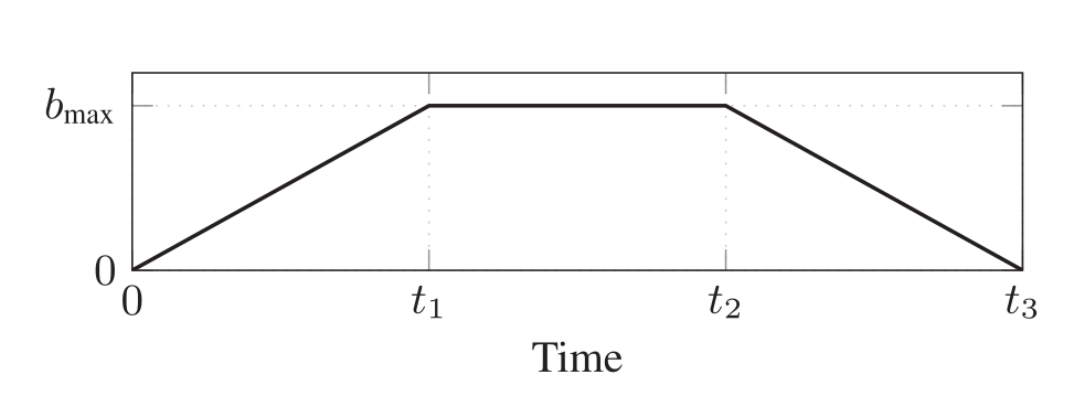
Time evolution of the external applied field

With \(t_1=5s\), \(t_2=10s\) and \(t_3=15s\)

11.1. Electric current density

The electric current density \(J_\theta\) is defined by :

\[ J_\theta=\sigma E = -\sigma \frac{\partial A_\theta}{\partial t}\]

With :

\[ \sigma = \frac{J_c}{E_c}\left(\frac{\mid\mid e\mid\mid}{E_c}\right)^{(1-n)/n}= \frac{J_c}{E_c}\left(\frac{\mid\mid -partial_t A_\theta\mid\mid}{E_c}\right)^{(1-n)/n}\]

Electric current density \(j_\theta (A/m^2)\)

We compare the current density profiles with FreeFEM and getDP on the \(O_r\) axis, at the mid-height of the cylinder, at time \(t_3\) for a maximum applied field of 1 T and \(n=20\), for a mesh of 30199 nodes.

L2 Relative Error Norm : \(35.84 \%\)

11.2. Magnetic flux density

The magnetic flux density \(B\) is defined by:

\[ B=\nabla\times A =\begin{pmatrix}-\partial_z A_\theta\\ 0\\ \frac{1}{r}\partial_r (rA_\theta)\end{pmatrix}\]

magnetic flux density magnitude \(B (T)\)

We compare the distribution of the z-component of the magnetic flux density 2mm above the cylinder at the instants \(t_1\), \(t_2\) and \(t_3\) with Feelpp and getDP.

t1 \(=5s\)

L2 Relative Error Norm : \(2.5 \%\)

t2 \(=10s\)

L2 Relative Error Norm : \(2.36 \%\)

t3 \(=15s\)

L2 Relative Error Norm : \(7.44 \%\)

12. References

Finite-Element Formulation for Systems with High-Temperature Superconductors, Julien Dular, Christophe Gauzaine, Benoît Vanderheyden, IEEE Transactions on Applied Superconductivity VOL. 30 NO. 3, April 2020, PDF