Test Case : getDP - Magnetostatic HTS with erf

1. Introduction

This is the test case of High-Temperature Superconductors with the A-V Formulation and Gauge Condition on a cylinder geometry surrounded by air in 2D coordinates.

2. Run the Calculation

The command line to run this case are :

    gmsh -2 -bin circle.geo
    getdp -m circle.msh circle2.pro -solve MagSta_a -pos MagSta

3. Data Files

The case data files are available in Github here :

PRO file - Edit the file
GEO file - Edit the file

4. Equation

The A-V Formulation in 2D coordinates with erf is :

A-V Formulation in 2D coordinates

\[ \begin{matrix} \Delta A_z = -\mu J & \text{on } \Omega & \text{(AV 2D)} \\ \end{matrix}\]

With :

\(A_{z}\) : \(z\) component of potential magnetic field
\(J=J_c \text{erf}\left(\frac{-A_z}{A_r}\right)\) : current density \(A/m^2\)
\(\mu\) : electric permeability \(kg/A^2/S^2\)

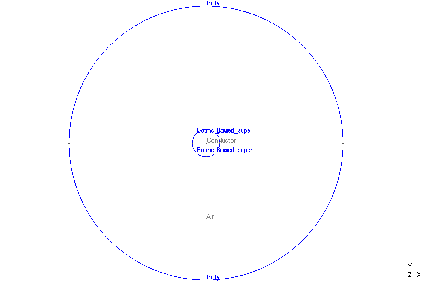
5. Geometry

The geometry is a circle in 2D coordinates \((x,y)\) representing a bulk cylinder, surrounded by air.

Geometry

The geometrical domains are :

Conductor : the cylinder
Air : the air surrounding Conductor
- Infty : the Air 's boundary

Symbol

Description

value

unit

\(R\)

radius of cylinder

\(0.001\)

\(R_{inf}\)

radius of infty border

\(0.01\)

6. Parameters

The parameters of the problem are :

On Conductor :

Symbol

Description

Value

Unit

\(\mu=\mu_0\)

magnetic permeability of vacuum

\(4\pi.10^{-7}\)

\(kg \, m / A^2 / S^2\)

\(A_r\)

parameter resulting from the combination of \(E_0\) and the time it takes to reach the peak of AC excitation

\(1.10^{-7}\)

\(Wb/m\)

\(b_{ext}\)

external applied field

\(0.02\)

\(T\)

\(J_c\)

critical current density

\(1.10^8\)

\(A/m^2\)

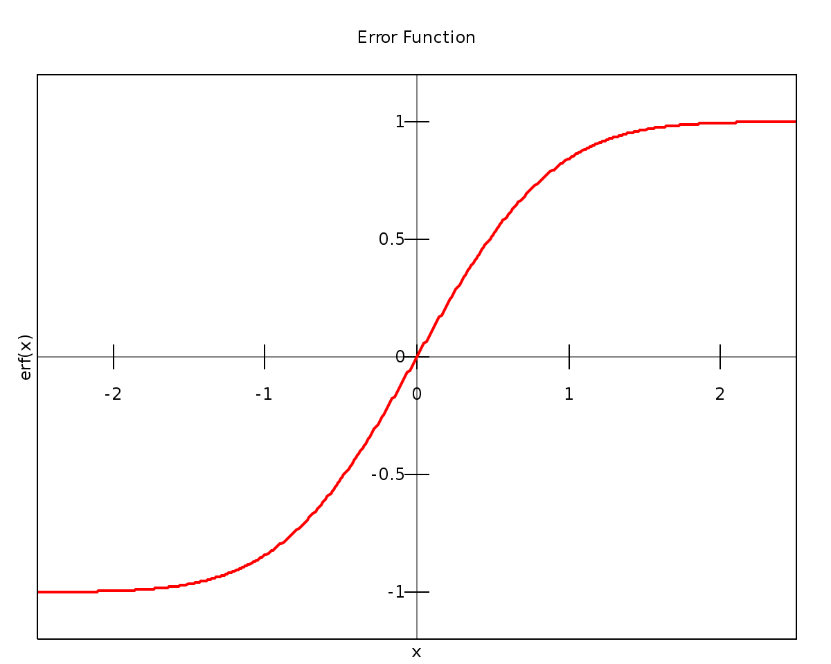
The error function erf is directly implemented on getDP :

\[erf(x)=\frac{2}{\sqrt{\pi}}\int_0^x \exp(-t^2)dt\]

On Air :

Symbol

Description

Value

Unit

\(\mu=\mu_0\)

magnetic permeability of vacuum

\(4\pi.10^{-7}\)

\(kg \, m / A^2 / S^2\)

On the PRO file, the parameters are written :

Parameters on PRO file

  mu0 = 4e-7 * Pi;
  DefineConstant [jc = {1e8, Name "Input/3Material Properties/2jc (Am⁻²)"}]; // Critical current density [A/m2]
  DefineConstant [Ar = {1e-7, Name "Input/3Material Properties/3Ar (Wb m^-1)"}];
  DefineConstant [bmax = {0.02, Name "Input/4Source/2Field amplitude (T)"}]; // Maximum applied magnetic induction [T]

  mu [ Air ]  =  mu0;
  mu [ Conductor ]  =  mu0;

  nu [ Air ]  = 1./ mu0;
  nu [ Conductor ]  = 1./ mu0;

  hmax[] = bmax;

7. Boundary Conditions

For the Dirichlet boundary conditions, we want to impose the applied magnetic field :

We have \(B_{max}=0.02 T\), and in 2D Cartesian coordinates, \(B=\nabla\times A\) becomes \(B_x=\partial A/\partial y\) and \(B_y=-\partial A/\partial x\). So in order to obtain a magnetic field \(B_{max}\) along \(y\), it is sufficient to impose \(A_z=-xB_{max}\).

Finally we have :

On Infty : \(A = -x B_{max}\)

On EDP file, the boundary conditions are written :

Boundary conditions on EDP file

Constraint {
    { Name Dirichlet_a_Mag;
        Case {
            { Region Gamma_e ; Value -X[]*hmax[]; }
        }
    }
}

8. Weak Formulation

Weak formulation of A Formulation in two dimensions approximation

\[ \int_{\Omega}{ - \frac{1}{\mu} \nabla A_z \cdot \nabla \phi \ dxdy } = \int_{\Omega_c}{ J_c erf\left(\frac{-A_z}{A_r}\right) \cdot \phi \ dxdy } + \int_{\Gamma_D}{ -B_0 x } \hspace{1cm} \text{(Weak A 2D)}\]

9. Implementation of the Weak Formulation

On getDP, we need to implement the Weak Formulation. The bilinear form was formulated as a non-linear problem, which in FreeFEM++ requires the source term to be multiplied by the unknown A. Hence, for the sake of consistency with the model, the source term is written as a reaction coefficient and multiplied by the term \((1/A)\).

First, the current density \(J\) is implemented :

J function on PRO file

    jfunc[] = jc * Erf[-CompZ[$1]/Ar]/((CompZ[$1] == 0) ? 1 : CompZ[$1]);
    js_fct[ Conductor ] = jfunc[$1];

Then on the PRO file, the weak formulation is written :

Weak Formulation on PRO file

Formulation {
  { Name Magnetostatics_a_2D; Type FemEquation;
    Quantity {
      { Name a ; Type Local; NameOfSpace Hcurl_a_Mag_2D; }
    }
    Equation {
      Integral { [  Dof{d a} , {d a} ];
        In Omega; Jacobian Vol; Integration Int; }
      Integral { [ -mu[] * js_fct[{a}]*Dof{a}, {a} ];
        In OmegaC; Jacobian Vol; Integration Int; }
  }
}

10. Mesh & Solver

Mesh

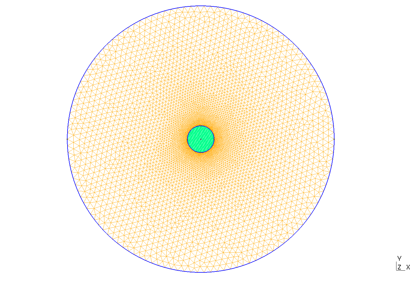
Mesh of Geometry

Non-linear Solver : Picard
- Maximum number of iterations : \(600\)

Solver on EDP file

Resolution {
  { Name MagSta_a;
    System {
      { Name Sys_Mag; NameOfFormulation Magnetostatics_a_2D; }
    }
    Operation {
      InitSolution[Sys_Mag];

      Generate[Sys_Mag]; GetResidual[Sys_Mag, $res0];
      Evaluate[ $res = $res0, $iter = 0 ];

      Print[{$iter, $res, $res / $res0},
        Format "Residual %03g: abs %14.12e rel %14.12e"];
      While[$res > NL_tol_abs && $res / $res0 > NL_tol_rel &&
            $res / $res0 <= 1 && $iter < NL_iter_max]{

        CopySolution[Sys_Mag,'x_Prev'];

        // Get the increment Delta_x
        Generate[Sys_Mag]; GetResidual[Sys_Mag, $res];
        Solve[Sys_Mag];
        CopySolution[Sys_Mag,'x_New'];
        AddVector[Sys_Mag, 1, 'x_New', -1, 'x_Prev', 'Delta_x'];

        AddVector[Sys_Mag, 1, 'x_New', NL_Relax, 'x_Prev', 'Delta_x'];
        CopySolution['x_New', Sys_Mag];
        Generate[Sys_Mag]; GetResidual[Sys_Mag, $res];

        Evaluate[ $iter = $iter + 1 ];
        Print[{$iter, $res, $res / $res0},
          Format "Residual %03g: abs %14.12e rel %14.12e"];
      }

      SaveSolution[Sys_Mag];

    }
  }
}

11. Results

The results that we obtain with this formulation with Feelpp are compared to the results of the article A numerical model to introduce student to AC loss calculation in superconductors where the finite element software FreeFEM is used.

11.1. Electric current density

The electric current density \(J\) is defined by :

\[ J= J_c \text{erf}\left(\frac{-A}{A_r}\right)\]

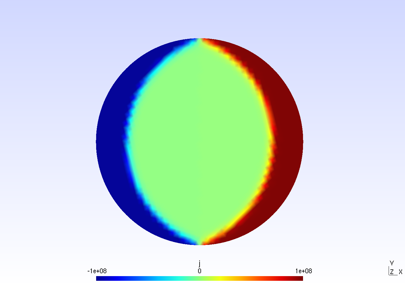
Figure 1. "Electric current density \(J (A/m^2)\)

We compare the current density profiles with getDP and FreeFEM on the \(O_r\) axis, on the diameter of the cylinder, for a maximum applied field of 0.02 T.

L2 Relative Error Norm : \(2.83 \%\)

11.2. Magnetic flux density

The magnetic flux density \(B\) is defined by:

\[ B=\nabla\times A =\begin{pmatrix}\partial_y A\\ -\partial_x A\\ 0\end{pmatrix}\]

Therefore, \(B_y\), the y-component of the magnetic flux density is defined as \(-\partial_x A\) :

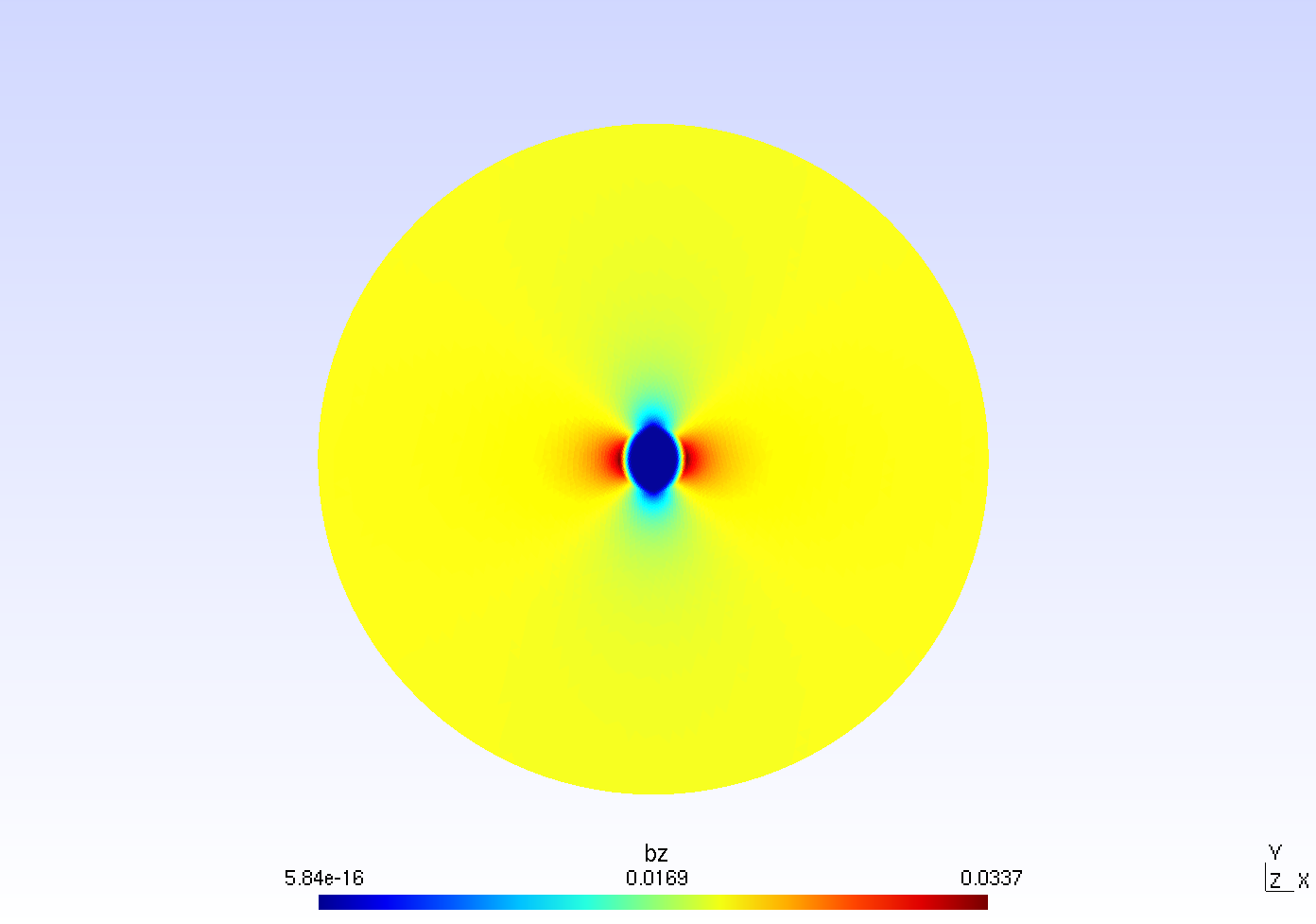
Figure 2. "y-component of the magnetic flux density \(B_y (T)\)

12. References

A numerical model to introduce students to AC loss calculation in superconductors. Francesco Grilli and Enrico Rizzo 2020 Eur. J. Phys. 41 045203