Test Case : Comsol - Pancake
1. Introduction
This is the test case of High-Temperature Superconductors with transport current using the T-A Formulation on a Pancake geometry surrounded by air in axisymmetric coordinates.
2. Run the Calculation
To run this case, compute the Study 1 solver on Comsol Multyphysics on the file TA_Axi.mph.
3. Data Files
The case data file is available on Github here.
4. Equation
The T-A Formulation in axysimmetric coordinates is :
With :
-
\(A_\theta\) : \(\theta\) component of potential magnetic field
-
\(T_r\) : \(r\) component of potential current density
-
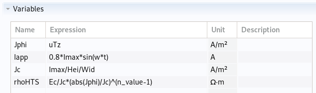
\(\rho\) : electric resistivity \(\Omega \cdot m\) defined by the E-J power law on HTS : \(\rho=\frac{E_c}{J_c}\left(\frac{\mid\mid J \mid\mid}{J_c}\right)^{(n)}=\frac{E_c}{J_c}\left(\frac{\mid\mid \partial_z T_r \mid\mid}{J_c}\right)^{(n)}\)
-
\(\mu\) : electric permeability \(kg/A^2/S^2\)
5. Geometry
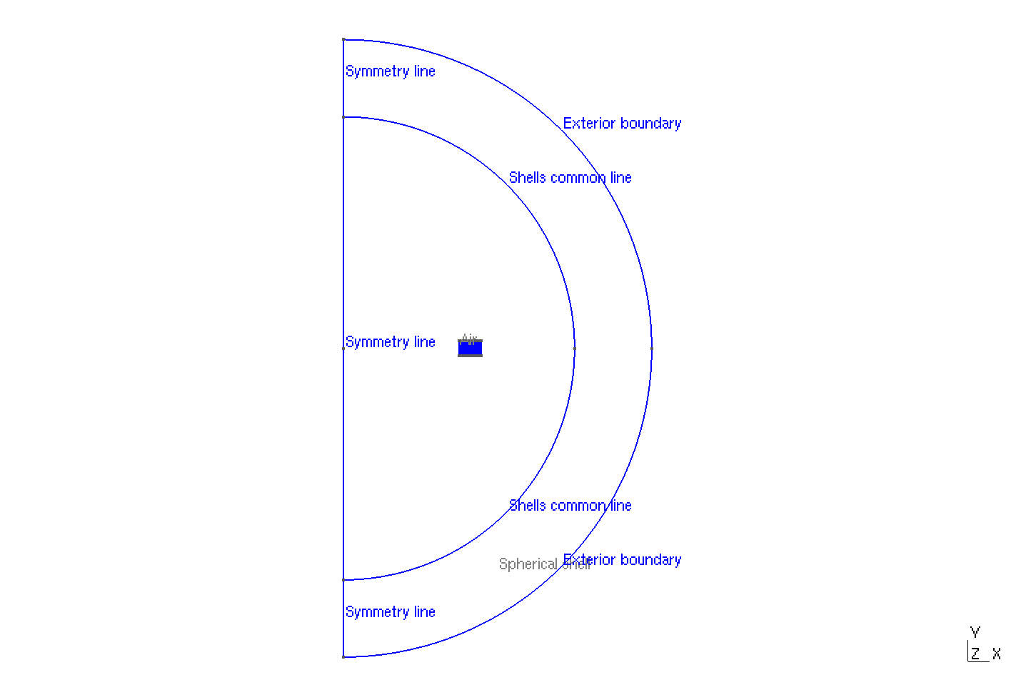
The geometry is a set of stacked tapes in axisymmetric coordinates \((r,z)\), surrounded by air. The geometry is created on Comsol, but in order to show the different physical names, this is a recreation on gmsh :
Geometry
|
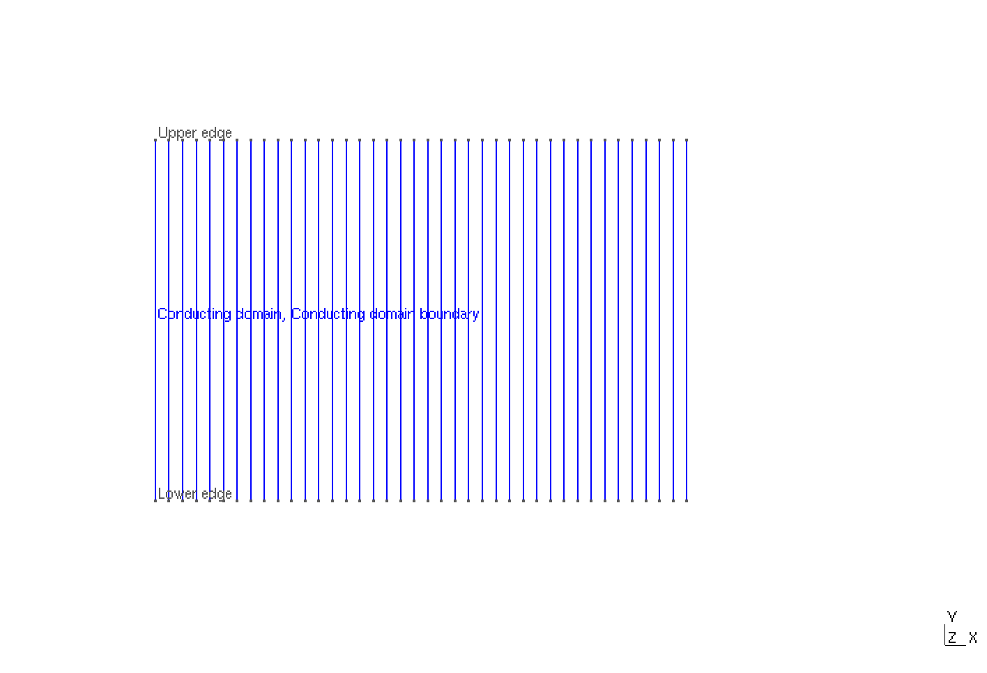
Zoom on Tapes
|
The geometrical domains are :
-
Conducting domain: the tapes-
Upper Edge: the top boundary of the tapes -
Lower Edge: the bottom boundary of the tapes -
Conducting domain boundary: the side boundaries of the tapes
-
-
Air: the air surroundingConductor-
Symmetry Line: the boundary for the symmetry in axisymmetric coordinates
-
-
Spherical Shell: the air surroundingConductor-
Exterior boundary: theSpherical Shell's boundary
-
Symbol |
Description |
value |
unit |
\(W_{tapes} (\delta)\) |
tapes width |
\(1e-6\) |
m |
\(H_{tapes}\) |
tapes height |
\(4e-3\) |
m |
\(step\) |
space between the tapes |
\(0.15e-3\) |
m |
\(R_{inf}\) |
radius of infty border |
\(0.08\) |
m |
6. Parameters
The parameters of the problem are :
-
On
Tapes:
Symbol |
Description |
Value |
Unit |
\(\mu=\mu_0\) |
magnetic permeability of vacuum |
\(4\pi.10^{-7}\) |
\(kg \, m / A^2 / S^2\) |
\(Wid\) |
tapes width |
\(1e-6\) |
\(m\) |
\(Hei\) |
tapes height |
\(4e-3\) |
\(m\) |
\(f\) |
frequency |
\(50\) |
\(Hz\) |
\(Imax\) |
max current |
\(120\) |
\(A\) |
\(Iapp\) |
applied current |
\(0.8*Imax*sin(2*\pi*f*t)\) |
\(A\) |
\(j_c\) |
critical current density |
\(3.10^{10}\) |
\(A/m^2\) |
\(e_c\) |
threshold electric field |
\(10^{-4}\) |
\(V/m\) |
\(n\) |
material dependent exponent |
\(40\) |
|
\(\rho\) |
electrical resistivity (described by the \(e-j\) power law) |
\(\frac{e_c}{j_c}\left(\frac{\mid\mid \partial_z T_r \mid\mid}{j_c}\right)^{(n)}\) |
\(\Omega\cdot m\) |
-
On
Air:
Symbol |
Description |
Value |
Unit |
\(\mu=\mu_0\) |
magnetic permeability of vacuum |
\(4\pi.10^{-7}\) |
\(kg \, m / A^2 / S^2\) |
On MPH file, the parameters are written :
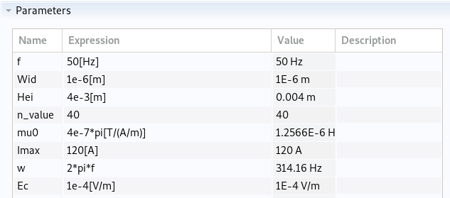
parameters
|
parameters
|
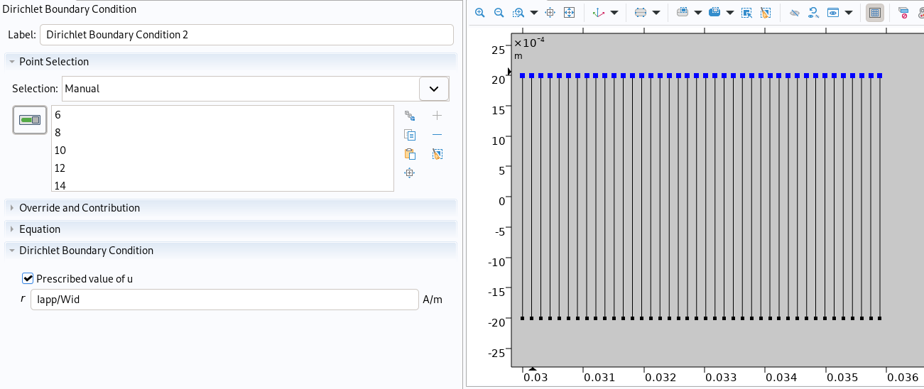
7. Boundary Conditions
For the Dirichlet boundary conditions, we want to impose the transport current :
The transport current is the difference of current potential between the top and the bottom of the tapes divided by the thickness of the tapes, so we can impose \(0\) at the bottom and \(Iapp/thickness\) at the top of the tapes.
Finally we have :
-
On
Top: \(T_r = Iapp/\delta\) -
On
Bottom: \(T_r = 0\)
On MPH file, the boundary conditions are written :
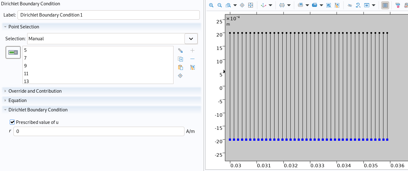
Dirichlet
|
Dirichlet
|
8. Weak Formulation
9. Ampere’s law & Coefficient Form PDE
For the A Formulation, the physic Magnetic Field (mf) is used on Comsol. It allows using the Ampère’s Law, which defined the A formulation :
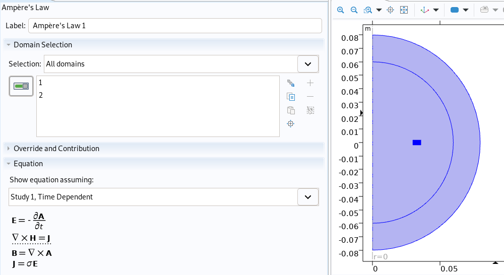
Ampère’s Law
|
The physic Coefficient Form PDE is used for the T Formulation. The coefficients associated to the Weak Formulation are :
-
On
Conducting domain:
Coefficient |
Description |
Expression |
\(c\) |
diffusion coefficient |
\(\begin{pmatrix} 0 & 0\\ 0 & -\rho \end{pmatrix}\) |
\(f\) |
source term |
\(-\mu_0\frac{\partial H}{\partial t}\) |
with \(H=\frac{1}{\mu_0}B\)
On MPH file, the coefficients are written :
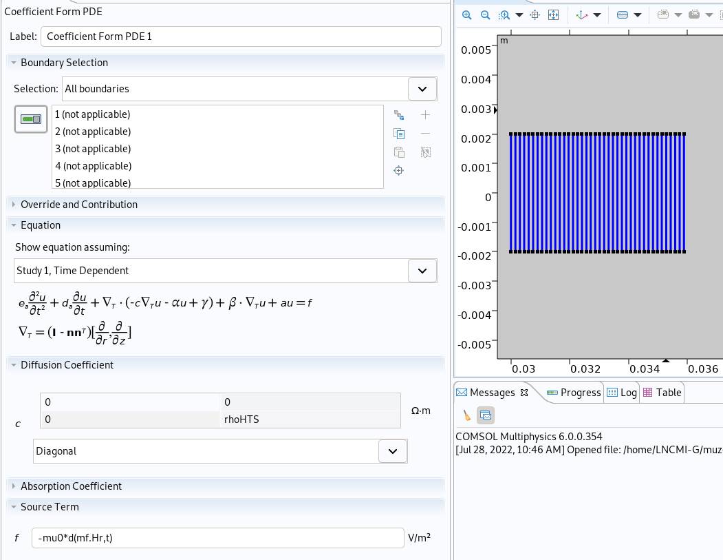
CFPDE
|
10. Numeric Parameters & Mesh
-
Time
-
Initial Time : \(0s\)
-
Final Time : \(0.02s\)
-
Time Step : \(2e-4s\)
-
-
Mesh
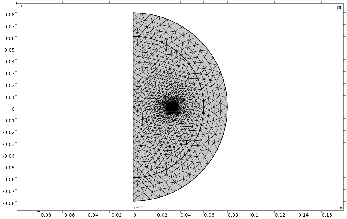
Mesh
|
11. Results
The results that we obtain with the T-A formulation with Comsol are compared to the results of the article COMSOL implementation of the H-φ-formulation with thin cuts for modeling superconductors with transport currents, where the solver Comsol is used with the H-φ Formulation.
11.1. Electric current density
The electric current density \(J\) is defined by :
We compare the current density profiles with the T-A formulation and the H-φ formulation on Comsol on the \(O_z\) axis, on the middle tape of the pancake, at time \(t=0.02s\) for a maximum applied current of 150 T and \(n=40\).
L2 Relative Error Norm : \(5.68 \%\) |
11.2. Magnetic flux density
The magnetic flux density \(B\) is defined by:
We can see that when the transport current is applied the tapes are generating a magnetic field, that stay trapped in the superconductor once the applied current is 0.
We compare the distribution of the r-component of the magnetic flux density with the T-A formulation and the H-φ formulation on Comsol on the \(Oz\) axis, in the middle of the pancake \(t=0.01s\).
L2 Relative Error Norm : \(0.94 \%\) |
12. References
-
Real-time simulation of large-scale HTS systems: multi-scale and homogeneous models using the T–A formulation, Edgar Berrospe-Juarez et al 2019 Supercond. Sci. Technol. 32 065003, PDF
-
COMSOL Implementation of the H-ϕ-Formulation With Thin Cuts for Modeling Superconductors With Transport Currents, A. Arsenault, B. d. S. Alves and F. Sirois, in IEEE Transactions on Applied Superconductivity, vol. 31, no. 6, pp. 1-9, Sept. 2021, Art no. 6900109, doi: 10.1109/TASC.2021.3097245. PDF