Test Case : Two Torus

1. Introduction

This is the test case of Maxwell Quasi Static Problem with the A-V Formulation and Gauge Condition on a two torus geometry surrounded by air for the unstationnary case in axisymmetric coordinates.

2. Run the Calculation

The command line to run this case is :

    mpirun -np 16 feelpp_toolbox_coefficientformpdes --config-file=mqs_axis.cfg --cfpdes.gmsh.hsize=1e-3

This case is run with the latest version 109 of Feelpp.

3. Data Files

The case data files are available in Github here :

CFG file - Edit the file
JSON file - Edit the file
GEO file - Edit the file

4. Equation

Assuming that \(V\) is known, the A-V Formulation in axisymmetric coordinates is :

A-V Formulation in axisymmetric coordinates

\[\text{(AV Axis)} \left\{ \begin{matrix} -\frac{1}{\mu}\Delta A_\theta + \frac{1}{\mu r^2}A_\theta + \sigma \frac{\partial A_\theta}{\partial t} + \frac{\sigma}{r} \frac{\partial V}{ \partial\theta}=0 & \text{on } \Omega^{axis} & \text{(AV-1 Axis)} \\ V = \frac{U}{2\pi} \, \theta & \text{ on } \Omega_c^{axis} & \text{(AV-2 Axis)} \\ A_{\theta} = 0 & \text{ on } \Gamma_D^{axis} & \text{(D Axis)} \\ \frac{\partial A_{\theta}}{\partial \mathbf{n}^{axis}} = 0 & \text{ on } \Gamma_N^{axis} & \text{(N Axis)} \end{matrix} \right.\]

With :

\(A_{\theta}\) : \(\theta\) component of potential magnetic field
\(\sigma\) : electric conductivity \(S/m\)
\(\mu\) : electric permeability \(kg/A^2/S^2\)
\(U\) : tension \(Volt\)

5. Geometry

The geometry is two rectangles in axisymmetric coordinates \((r,z)\) representing two conducting torus, surrounded by air.

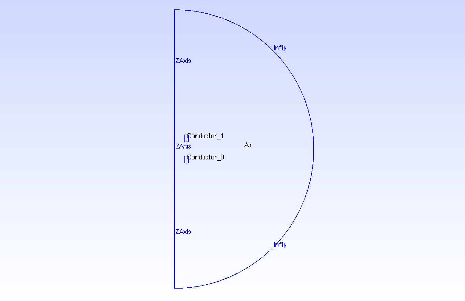
Geometry in Axisymmetrical cut

Geometry in Axisymmetrical cut loop on Conductors

The geometrical domains are :

Conductor_0 : the torus is composed by a conductor
Conductor_1 : the torus is composed by a conductor

Conductor_0 \(\cup\) Conductor_1 \( = \Omega_c^{axis}\)

Air : the air surrounding Conductor_0 and Conductor_1
- zAxis : Air 's bound, correspond to \(Oz\) axis (\(\{(z,r), \, z=0 \}\))
- infty : the rest of the Air 's bound

Air \(= \Omega^{axis} / \Omega_c^{axis}\).

Symbol

Description

value

unit

\(r_{int}\)

interior radius of tores

\(75e-3\)

\(r_{ext}\)

exterior radius of tores

\(100.2e-3\)

\(z_1\)

half-height of tores

\(25e-3\)

\(r_{infty}\)

radius of infty border

\(5*r_{ext}\)

6. Boundary Conditions

The Dirichlet boundary conditions imposed are :

On zAxis : \(A_{\theta} = 0\)
On infty : \(A_{\theta} = 0\)

On JSON file, the boundary conditions are written :

Boundary conditions on JSON file

    "BoundaryConditions":
    {
        "magnetic":
        {
            "Dirichlet":
            {
                "ZAxis":
                {
                    "expr":"0"
                },
                "Infty":
                {
                    "expr":"0"
                }
            }
        }
    }

7. Weak Formulation

Weak Formulation

\[\scriptsize{ \int_{\Omega^{axis}}{ \frac{r}{\mu} \tilde\nabla A_\theta \cdot \tilde\nabla \phi \ drdz } + \int_{\Omega^{axis}}{\frac{1}{\mu r} A_\theta \cdot \phi \ drdz} +\int_{\Omega^{axis}}{ \sigma r \frac{\partial A_\theta}{\partial t} \cdot \phi \ drdz} = \int_{\Omega^{axis}_c}{ \sigma \frac{\partial V}{\partial \theta} \cdot\phi \ rdrdz } }\]

With \(\tilde{\nabla} = \begin{pmatrix} \partial r \\ \partial z \end{pmatrix}\)

8. Parameters

The parameters of the problem are :

On Conductor_0 and Conductor_1 :

Symbol

Description

Value

Unit

\(V_0\)

scalar electrical potential of Conductor_0

\( U_0 \, \frac{\theta}{2\pi}\)

\(Volt\)

\(U_0\)

electrical potential of Conductor_0

\(\begin{cases} \frac{t}{0.1} \quad\text{if } t <0.1 \\ 1 \quad\text{if } 0.1<t<0.5 \\ 0 \quad\text{if } 0.5<t<1 \end{cases}\)

\(Volt / rad\)

\(V_1\)

scalar electrical potential of Conductor_1

\( U_1 \, \frac{\theta}{2\pi}\)

\(Volt\)

\(U_1\)

electrical potential of Conductor_1

\(\begin{cases} \frac{t}{0.1} \quad\text{if } 0 < t < 0.1 \\ 1 \quad\text{if } 0.1 < t < 0.7 \\ 0 \quad\text{if } 0.7 < t < 1 \end{cases}\)

\(Volt / rad\)

\(\sigma\)

electrical conductivity

\(58e6\)

\(S/m\)

\(\mu=\mu_0\)

magnetic permeability of vacuum

\(4\pi.10^{-7}\)

\(kg \, m / A^2 / S^2\)

On Air :

Symbol

Description

Value

Unit

\(\mu=\mu_0\)

magnetic permeability of vacuum

\(4\pi.10^{-7}\)

\(kg \, m / A^2 / S^2\)

On JSON file, the parameters are written :

Parameters on JSON file

    "Parameters":
    {
        "sigma":58e6,
	    "mu":"4*pi*1e-7"
    },
    "Materials":
    {
        "Conductor_0":
        {
            "U":"t/(0.1)*(t<(0.1))+(t<(0.5))*(t>(0.1)):t",
	        //[...]
        },
        "Conductor_1":
        {
            "U":"t/(0.1)*(t<(0.1))+(t<(0.7))*(t>(0.1)):t",
	        //[...]
        },
        "Air":
        {
            //[...]
        }
    },

9. Coefficient Form PDEs

The Feelpp toolboxe Coefficient Form PDEs is used here. The coefficients associated to the Weak Formulation are :

On Conductor_0 and Conductor_1 :

Coefficient

Description

Expression

\(d\)

damping or mass coefficient

\(\sigma r\)

\(c\)

diffusion coefficient

\(\frac{r}{\mu}\)

\(a\)

absorption or reaction coefficient

\(\frac{1}{\mu r}\)

\(f\)

source term

\(- \sigma \frac{U_i}{2\pi} \, r\) with \(i={0,1}\)

On Air :

Coefficient

Description

Expression

\(c\)

diffusion coefficient

\(\frac{r}{\mu}\)

\(a\)

absorption or reaction coefficient

\(\frac{1}{\mu r}\)

On JSON file, the coefficients are written :

CFPDEs coefficients on JSON file

    "Materials":
    {
        "Conductor_0":
        {
            "U":"t/(0.1)*(t<(0.1))+(t<(0.5))*(t>(0.1)):t",
	        "magnetic_c":"x/mu:x:mu",
            "magnetic_a":"1/mu/x:mu:x",
            "magnetic_f":"-sigma*U/2/pi:sigma:U",
            "magnetic_d":"sigma*x:sigma:x"
        },
        "Conductor_1":
        {
            "U":"t/(0.1)*(t<(0.1))+(t<(0.7))*(t>(0.1)):t",
	        "magnetic_c":"x/mu:x:mu",
            "magnetic_a":"1/mu/x:mu:x",
            "magnetic_f":"-sigma*U/2/pi:sigma:U",
            "magnetic_d":"sigma*x:sigma:x"
        },
        "Air":
        {
            "magnetic_c":"x/mu:x:mu",
            "magnetic_a":"1/mu/x:mu:x"
        }
    }

10. Numeric Parameters

Time
- Initial Time : \(0s\)
- Final Time : \(1s\)
- Time Step : \(0.01s\)
Mesh size :
- Interior of torus : \(0.001 m\)
- Far of torus : \(0.004 m\)

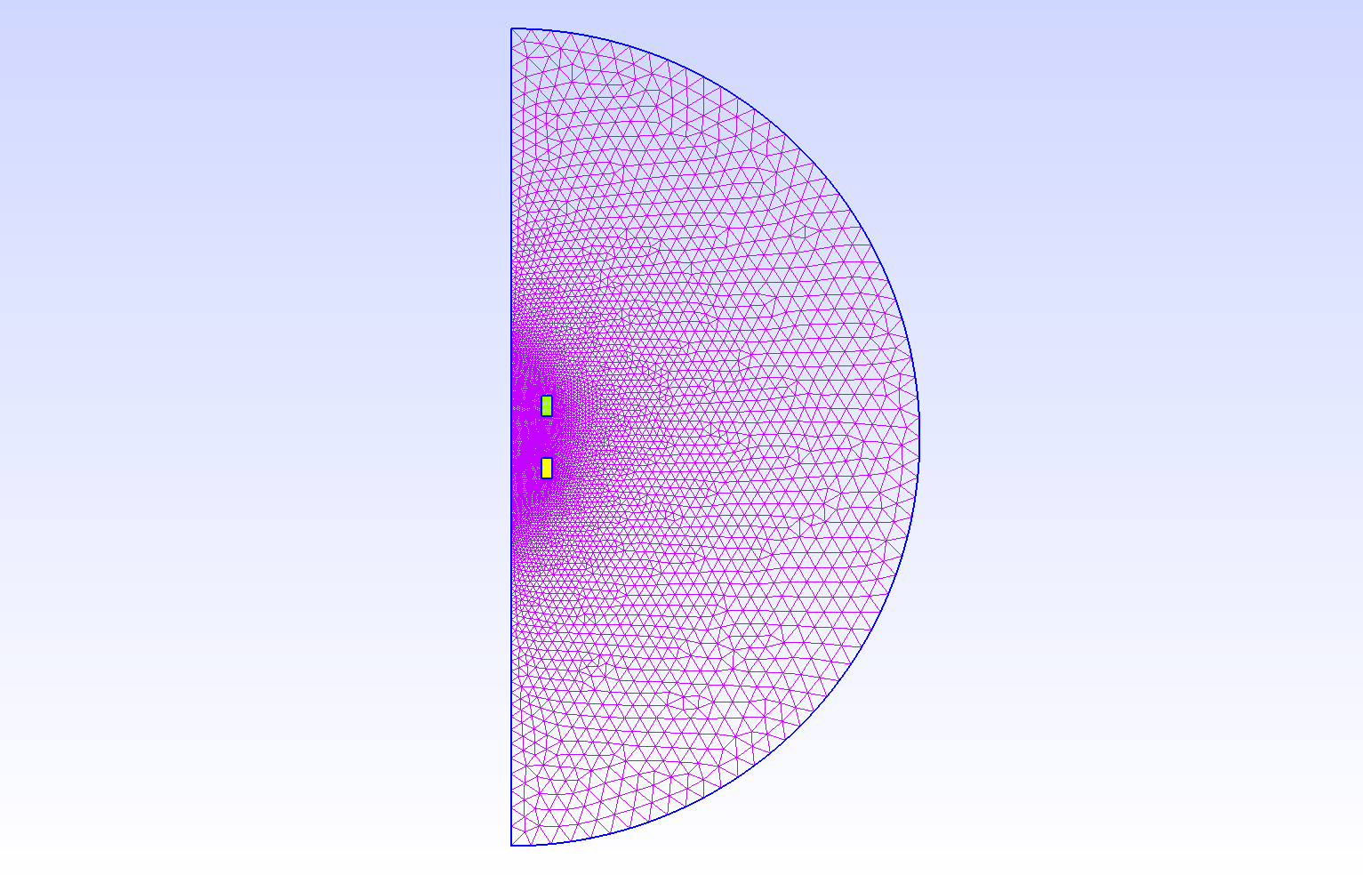
Mesh of Geometry

11. Result

11.1. Magnetic Potential Field

The magnetic potential field \(\mathbf{A}\) defined by :

\[ \mathbf{A} = \begin{pmatrix} 0 \\ A_{\theta} \\ 0 \end{pmatrix}_{cyl}\]

\(\theta\) component of Magnetic potential field \(A_\theta (A/m^2)\)

11.2. Magnetic Field

The magnetic field \(\mathbf{B}\) is defined by :

\[ \mathbf{B} = \nabla \times \mathbf{A} = \begin{pmatrix} -\partial_z A_\theta \\ 0 \\ \frac{1}{r}\partial_r (rA_\theta) \end{pmatrix}_{cyl}\]

\(r\) component of Magnetic field \(B_r (T)\)

\(z\) component of Magnetic field \(B_z (T)\)

The behavior of \(\mathbf{B}_z\) on the \(O_z\) axis at \(t=15s\) :

Table 1. L2 Error Norm for \(B_z\) on \(O_z\) at \(t=15s\)
h	L2 Error Norm	L2 Relative Error Norm
\(9e-3\)	\(4.235206e-2\)	\(1.84\%\)
\(5e-3\)	\(2.294347e-2\)	\(1.00\%\)
\(1e-3\)	\(3.908771e-3\)	\(0.17\%\)
\(5e-4\)	\(1.292564e-3\)	\(0.06\%\)