Test Case : FreeFEM - Magnetostatic HTS with erf

1. Introduction

This is the test case of High-Temperature Superconductors with the A-V Formulation and Gauge Condition on a bulk cylinder geometry surrounded by air in 2D coordinates corresponding to the paper A numerical model to introduce students to AC loss calculation in superconductors by Francesco Grilli and Enrico Rizzo.

2. Run the Calculation

The command line to run this case is :

    ff-mpirun -np 4 round_magn.edp -wg

3. Data Files

The case data files are available in Github here :

EDP file - Edit the file

4. Equation

The A-V Formulation in 2D coordinates with erf is :

A-V Formulation in 2D coordinates

\[ \begin{matrix} \Delta A_z = -\mu J & \text{on } \Omega & \text{(AV 2D)} \\ \end{matrix}\]

With :

\(A_{z}\) : \(z\) component of potential magnetic field
\(J=J_c \text{erf}\left(\frac{-A_z}{A_r}\right)\) : current density \(A/m^2\)
\(\mu\) : electric permeability \(kg/A^2/S^2\)

5. Geometry

The geometry is a circle in 2D coordinates \((x,y)\) representing a bulk cylinder, surrounded by air.

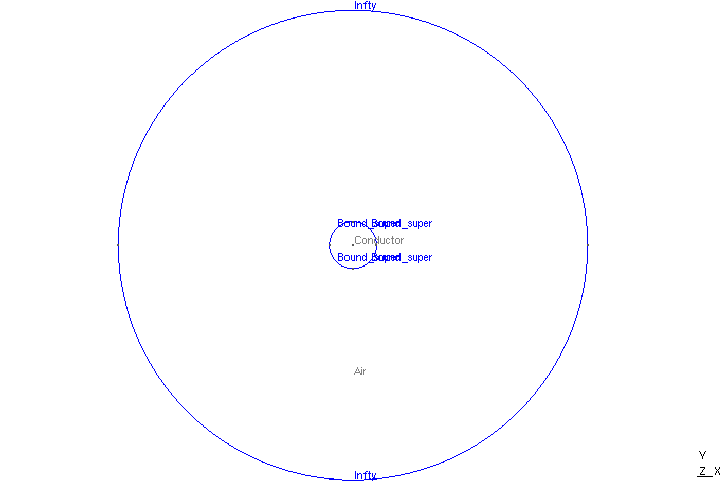
Geometry

The geometrical domains are :

Conductor : the cylinder
Air : the air surrounding Conductor
- Infty : the Air 's boundary

Symbol

Description

value

unit

\(R\)

radius of cylinder

\(0.001\)

\(R_{inf}\)

radius of infty border

\(0.01\)

6. Parameters

The parameters of the problem are :

On Conductor :

Symbol

Description

Value

Unit

\(\mu=\mu_0\)

magnetic permeability of vacuum

\(4\pi.10^{-7}\)

\(kg \, m / A^2 / S^2\)

\(A_r\)

parameter resulting from the combination of \(E_0\) and the time it takes to reach the peak of AC excitation

\(1.10^{-7}\)

\(Wb/m\)

\(b_{ext}\)

external applied field

\(0.02\)

\(T\)

\(J_c\)

critical current density

\(1.10^8\)

\(A/m^2\)

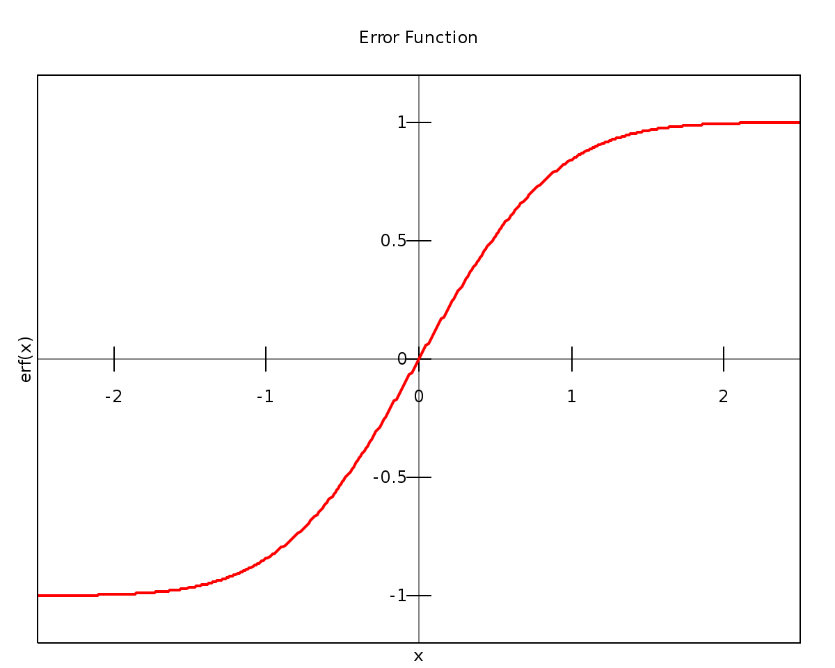
The error function erf is directly implemented on FreeFEM :

\[erf(x)=\frac{2}{\sqrt{\pi}}\int_0^x \exp(-t^2)dt\]

On Air :

Symbol

Description

Value

Unit

\(\mu=\mu_0\)

magnetic permeability of vacuum

\(4\pi.10^{-7}\)

\(kg \, m / A^2 / S^2\)

On EDP file, the parameters are written :

Parameters on EDP file

    // Applied field, in tesla
    real Bext=0.02, theta=0;
    // Coefficients
    real Jc=1e8, Ar=1e-7, mu=4e-7*pi;

7. Boundary Conditions

For the Dirichlet boundary conditions, we want to impose the applied magnetic field :

We have \(B_{ext}=0.02 T\), and in 2D Cartesian coordinates, \(B=\nabla\times A\) becomes \(B_x=\partial A/\partial y\) and \(B_y=-\partial A/\partial x\). So in order to obtain a magnetic field \(B_{ext}\) along \(y\), it is sufficient to impose \(A_z=-xB_{ext}\).

Finally we have :

On Infty : \(A = -x B_{ext}\)

On the EDP file, the boundary conditions are written :

Boundary conditions on EDP file

    // Boundary conditions
    func bc=Bext*(-x);

8. Weak Formulation

Weak formulation of A Formulation in two dimensions approximation

\[ \int_{\Omega}{ - \frac{1}{\mu} \nabla A_z \cdot \nabla \phi \ dxdy } = \int_{\Omega_c}{ J_c erf\left(\frac{-A_z}{A_r}\right) \cdot \phi \ dxdy } + \int_{\Gamma_D}{ -B_0 x } \hspace{1cm} \text{(Weak A 2D)}\]

9. Implementation of the Weak Formulation

On FreeFEM, we need to implement the Weak Formulation. The bilinear form was formulated as a non-linear problem, which in FreeFEM++ requires the source term to be multiplied by the unknown A. Hence, for the sake of consistency with the model, the source term is written as a reaction coefficient and multiplied by the term \((1/A)\).

On the EDP file, the weak formulation is written :

Weak Formulation on EDP file

    // Finite element space and problem definition
    fespace Vh(Th,P2);                                          // Fespace defined over the triangulation Th, with 2nd order polynomials as test function
    Vh u,uu=1,ue=1,v;                                           // u --> unknown
                                                                // uu --> variable for the non linear function
                                                                // ue --> variable to store the solution of the (i-1)th iteration
                                                                // v --> test function
    Vh fd=1*(region==sc) + 0*(region==air);                     // Dependence upon the region (i.e. air or conductor) defined within the fespace

    macro Grad(u)[dx(u),dy(u)]//                                // Macro for bilinear form in array-format

    // Non linear function
    macro F(h) (mu*Jc*fd*erf(-h/Ar))/h//                        // Macro for the nonlinear function (only on conductor)

    // Problem definition
    problem Aform(u,v) = int2d(Th)(Grad(u)'*Grad(v))            // on air & conductor
                        - int2d(Th)(u*F(uu)*v)                  // on conductor
                        + on(D,u=bc);                           // Dirichlet boundary condition

10. Mesh & Solver

Mesh

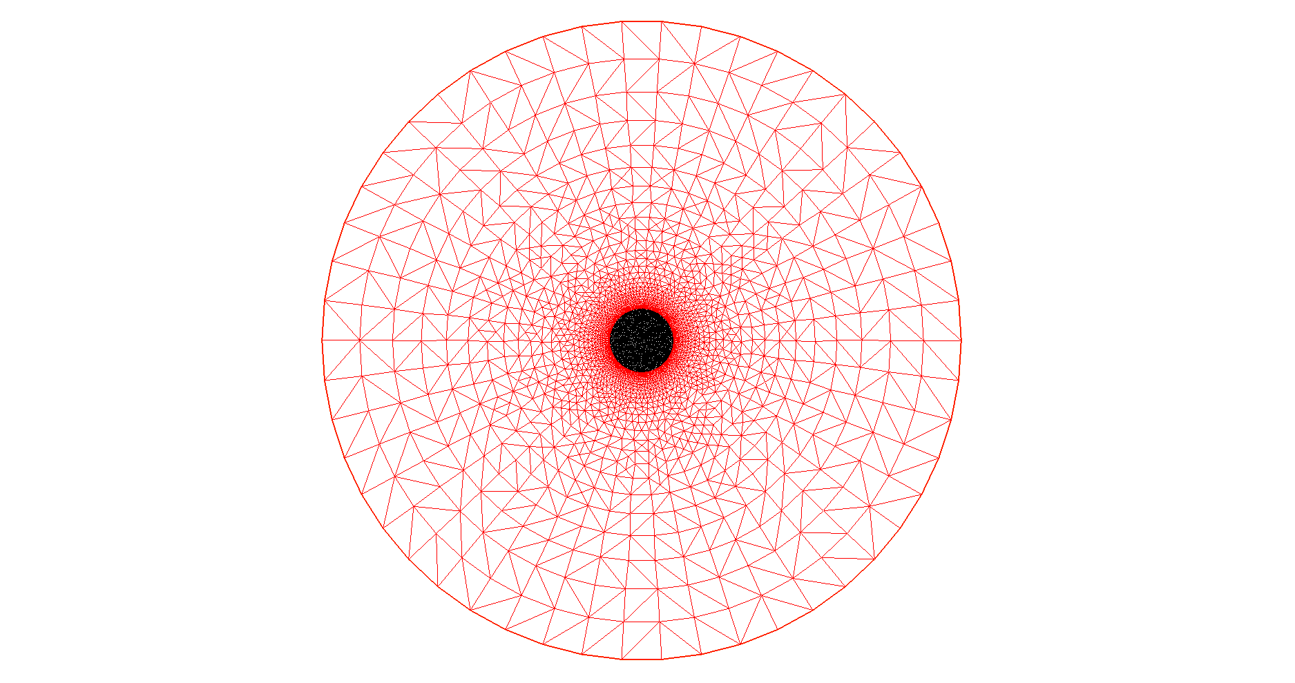
Mesh of Geometry

Non-linear Solver : Picard

Solver on EDP file

while (abs(err)>=toll) {
    Aform;
    uu=u;                                                      // Set the argument of the non linear function

    err=(abs(u(0,0)-ue(0,0)))/(u(0,0));                        // Residuals evaluation/ convergence at (x,y)=(0,0)
    cout<<"Convergence at (x,y)=(0,0), err:"<< err << endl;    // Plot error
    Residuals<<"    "<<   i   <<"    "<<   err   <<endl;

    ue=u;                                                      // Value update
    i++;
}

11. Results

11.1. Electric current density

The electric current density \(J\) is defined by :

\[ J= J_c \text{erf}\left(\frac{-A}{A_r}\right)\]

Figure 1. "Electric current density \(J (A/m^2)\)

The behaviour of \(J\) on the \(O_r\) axis, on the diameter of the cylinder, for a maximum applied field of 0.02 T is :

11.2. Magnetic flux density

The magnetic flux density \(B\) is defined by:

\[ B=\nabla\times A =\begin{pmatrix}\partial_y A\\ -\partial_x A\\ 0\end{pmatrix}\]

Therefore, \(B_y\), the y-component of the magnetic flux density is defined as \(-\partial_x A\) :

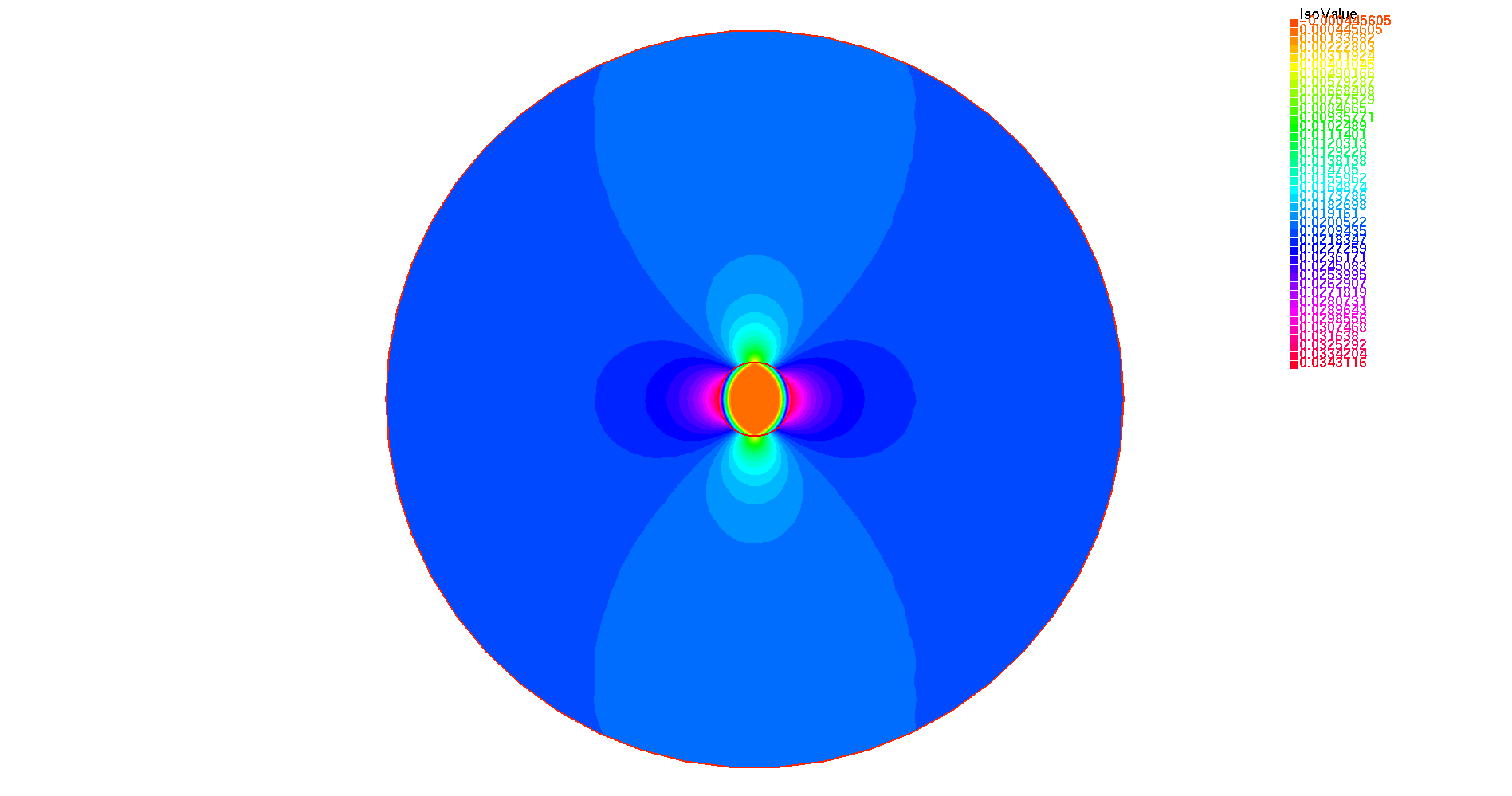
Figure 2. "y-component of the magnetic flux density \(B_y (T)\)

12. References

A numerical model to introduce students to AC loss calculation in superconductors. Francesco Grilli and Enrico Rizzo 2020 Eur. J. Phys. 41 045203