Test Case : Comsol - Stacked tapes
1. Introduction
This is the test case of High-Temperature Superconductors with transport current using the T-A Homogeneous Formulation on stacked tapes geometry surrounded by air in axisymmetric coordinates given with the article Real-time simulation of large-scale HTS systems: multi-scale and homogeneous models using the T–A formulation, Edgar Berrospe-Juarez et al 2019 Supercond.
2. Run the Calculation
To run this case, compute the Study 1 solver on Comsol Multyphysics on the file Bench03_TA_Hom.mph.
3. Data Files
The case data file is available on Github here.
4. Equation
The T-A Homogeneous Formulation in axysimmetric coordinates is :
With :
-
\(A_\theta\) : \(\theta\) component of potential magnetic field
-
\(T_r\) : \(r\) component of potential current density
-
\(\rho\) : electric resistivity \(\Omega \cdot m\) defined by the E-J power law on HTS : \(\rho=\frac{E_c}{J_c}\left(\frac{\mid\mid J \mid\mid}{J_c}\right)^{(n)}=\frac{E_c}{J_c}\left(\frac{\mid\mid \partial_z T_r \mid\mid}{J_c}\right)^{(n)}\)
-
\(\mu\) : electric permeability \(kg/A^2/S^2\)
-
\(\delta\) : thickness of the tapes \(m\)
-
\(\Lambda\) : space between the Tapes \(m\)
5. Geometry
The geometry is a set of stacked tapes in axisymmetric coordinates \((r,z)\), surrounded by air. The geometry is created on Comsol, but in order to show the different physical names, this is a recreation on gmsh :
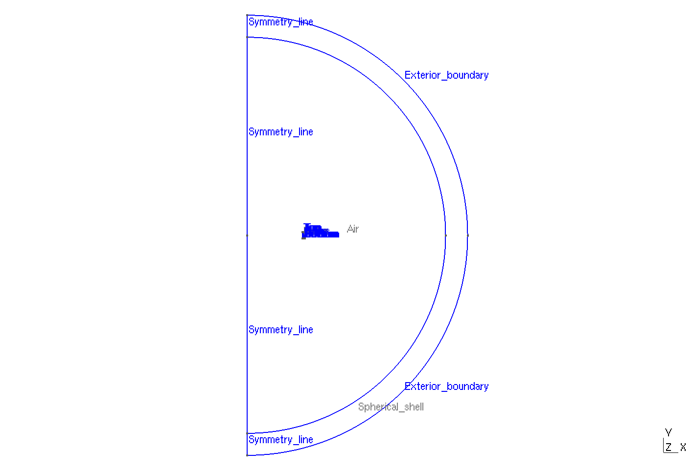
Geometry
|
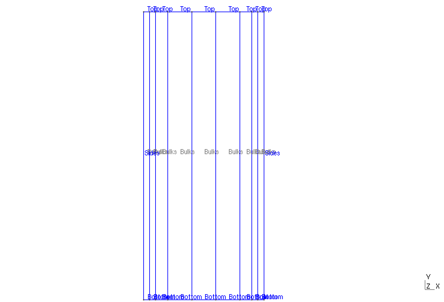
Zoom on Tapes
|
The geometrical domains are :
-
Bulks: the tapes represented by bulks for the Homogeneous approach-
Top: the top boundary of the tapes -
Bottom: the bottom boundary of the tapes -
Sides: the side boundaries of the tapes
-
-
Air: the air surroundingConductor-
Symmetry Line: the boundary for the symmetry in axisymmetric coordinates
-
-
Spherical Shell: the air surroundingConductor-
Exterior boundary: theSpherical Shell's boundary
-
Symbol |
Description |
value |
unit |
\(W_{tapes} (\delta)\) |
tapes width |
\(1e-6\) |
m |
\(H_{tapes}\) |
tapes height |
\(12e-3\) |
m |
\(cel_{tapes} (\Lambda)\) |
space between the tapes |
\(250e-6\) |
m |
\(R_{inf}\) |
radius of infty border |
\(0.4\) |
m |
6. Parameters
The parameters of the problem are :
-
On
Bulks:
Symbol |
Description |
Value |
Unit |
\(\mu=\mu_0\) |
magnetic permeability of vacuum |
\(4\pi.10^{-7}\) |
\(kg \, m / A^2 / S^2\) |
\(thickness_{tape}\) |
tapes width |
\(1e-6\) |
\(m\) |
\(thickness_{cell}\) |
space between the tapes |
\(250e-6\) |
\(m\) |
\(height\) |
tapes height |
\(12e-3\) |
\(m\) |
\(f\) |
frequency |
\(50\) |
\(Hz\) |
\(Ic\) |
critical current |
\(300\) |
\(A\) |
\(Iapp\) |
applied current |
\(0.5*Ic*sin(2*\pi*f*t)\) |
\(A\) |
\(j_c\) |
critical current density |
\(2.5.10^10\) |
\(A/m^2\) |
\(e_c\) |
threshold electric field |
\(10^{-4}\) |
\(V/m\) |
\(n\) |
material dependent exponent |
\(25\) |
|
\(\rho\) |
electrical resistivity (described by the \(e-j\) power law) |
\(\frac{e_c}{j_c}\left(\frac{\mid\mid \partial_z T_r \mid\mid}{j_c}\right)^{(n)}\) |
\(\Omega\cdot m\) |
-
On
Air:
Symbol |
Description |
Value |
Unit |
\(\mu=\mu_0\) |
magnetic permeability of vacuum |
\(4\pi.10^{-7}\) |
\(kg \, m / A^2 / S^2\) |
On MPH file, the parameters are written :
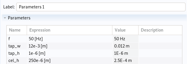
parameters
|
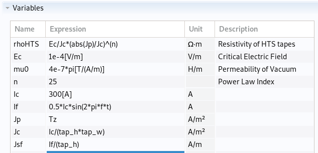
parameters
|
7. Boundary Conditions
For the Dirichlet boundary conditions, we want to impose the transport current :
The transport current is the difference of current potential between the top and the bottom of the tapes divided by the thickness of the tapes, so we can impose \(0\) at the bottom and \(Iapp/thickness\) at the top of the tapes
Finally we have :
-
On
Top: \(T_r = Iapp/\delta\) -
On
Bottom: \(T_r = 0\)
For the Neumann boundary conditions, the homogeneous approach of the T-A formulation impose that it is \(0\) on both side of the bulk representation.
Finally we have :
-
On
Sides: \(T_r \cdot \mathbf{n} = 0\)
On MPH file, the boundary conditions are written :
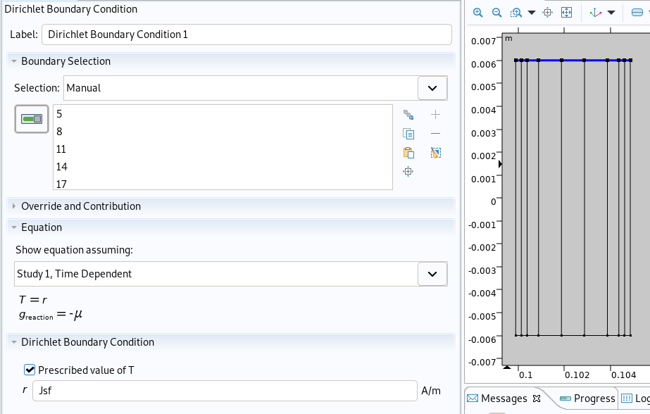
Dirichlet
|
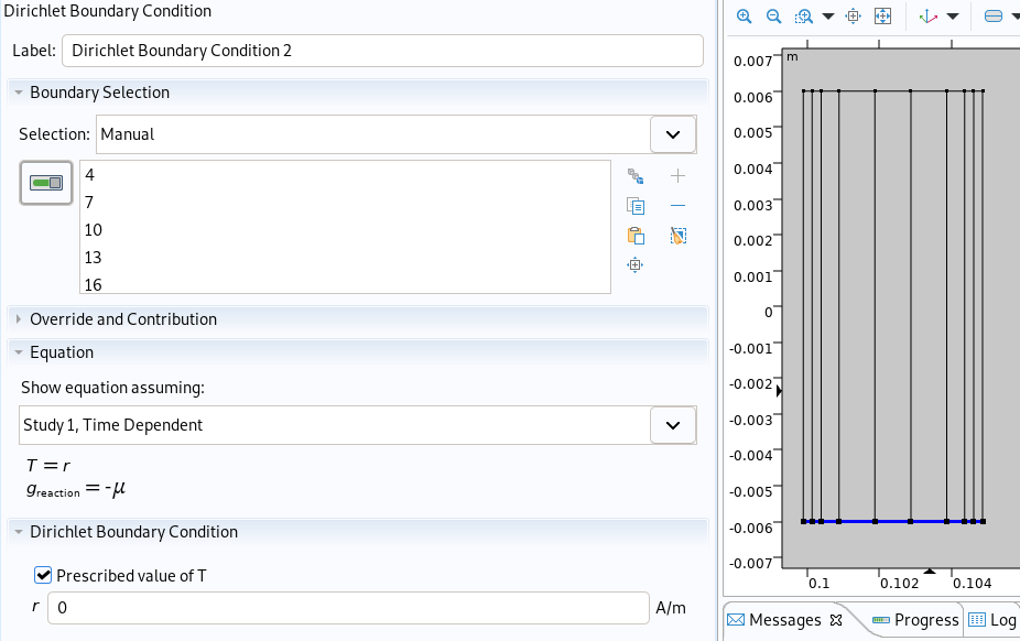
Dirichlet
|
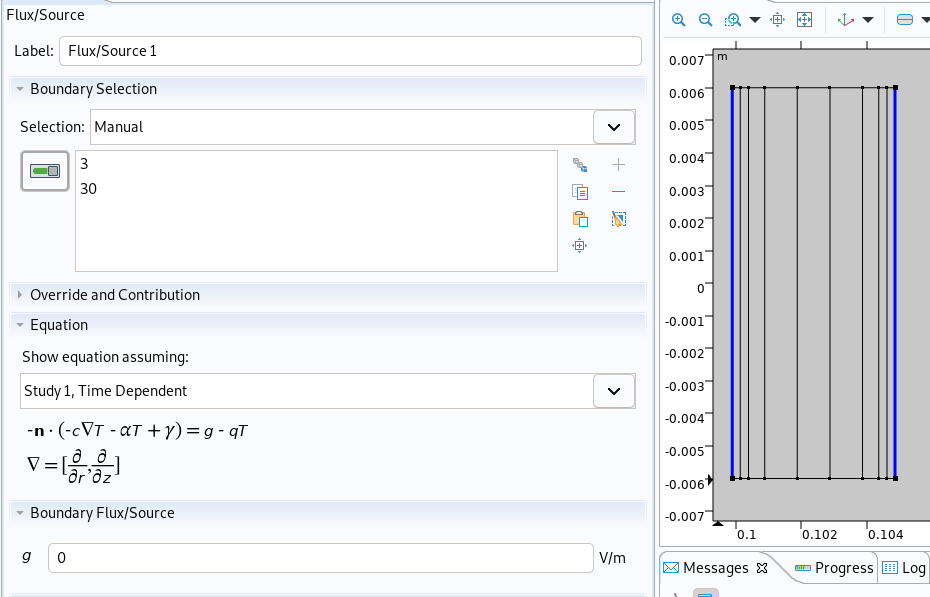
Neumann
|
8. Weak Formulation
9. Ampere’s law & Coefficient Form PDE
For the A Formulation, the physic Magnetic Field (mf) is used on Comsol. It allows using the Ampère’s Law, which defined the A formulation :
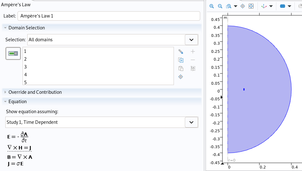
Ampère’s Law
|
The physic Coefficient Form PDE is used for the T Formulation. The coefficients associated to the Weak Formulation are :
-
On
Bulks:
Coefficient |
Description |
Expression |
\(c\) |
diffusion coefficient |
\(\begin{pmatrix} 0 & 0\\ 0 & -\rho \end{pmatrix}\) |
\(f\) |
source term |
\(-\mu_0\frac{\partial H}{\partial t}\) |
with \(H=\frac{1}{\mu_0}B\)
On MPH file, the coefficients are written :
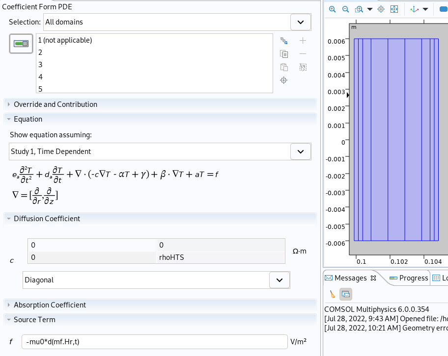
CFPDE
|
10. Numeric Parameters & Mesh
-
Time
-
Initial Time : \(0s\)
-
Final Time : \(0.02s\)
-
Time Step : \(2e-4s\)
-
-
Mesh
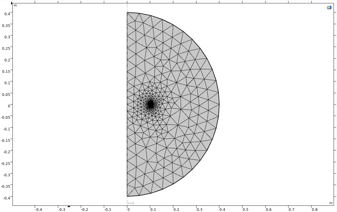
Mesh
|
11. Results
The results that we obtain with the T-A Homogeneous formulation with Comsol are of featured file of the results of the article Real-time simulation of large-scale HTS systems: multi-scale and homogeneous models using the T–A formulation.
The time evolution of the applied current is :
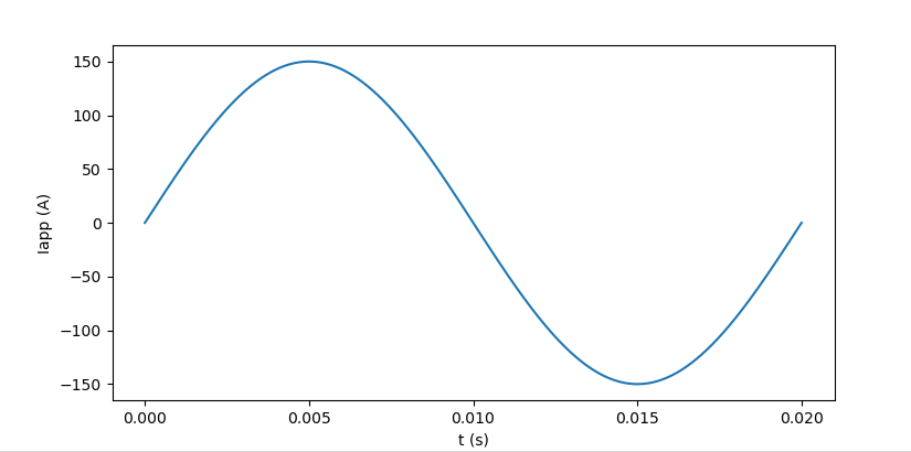
Time evolution of the applied current
|
11.1. Electric current density
The electric current density \(j_\theta\) is defined by :
The distribution of the electric current density on the Oz axis between the tapes at \(t=0.005s\) with Comsol is :
11.2. Magnetic flux density
The magnetic flux density \(B\) is defined by:
As such, \(B_r=-\partial_z A_\theta\) and \(B_z=\frac{1}{r}\partial_r (rA_\theta)\) :
The distribution of the r-component of the magnetic flux density on the Oz axis between the tapes at the instant \(t=0.005s\) with * Comsol is :
The distribution of the z-component of the magnetic flux density on the Or axis across the tapes at the instant \(t=0.005s\) with Comsol is :
12. References
-
Real-time simulation of large-scale HTS systems: multi-scale and homogeneous models using the T–A formulation, Edgar Berrospe-Juarez et al 2019 Supercond. Sci. Technol. 32 065003, PDF