Test Case of Thermo-Elasto-Magnetism in Transient Case and Axisymmetrical Coordinates

1. Introduction

This page presents the simulation and results of based on the theory Elastic Equations with Electromagnetism and Thermic in Axisymmetrical case : Elastic and Thermo-Electromagnetism problem coupled by Laplace Force and Thermal Dilatation in transient case and axisymmetric coordinates.

2. Run the calculation

The command line to run this case is :

    mpirun -np 16 feelpp_toolbox_coefficientformpdes --config-file=elasto-thermo-mag.cfg --cfpdes.gmsh.hsize=5e-3

To compute with the Laplace Force and the Thermal Dilatation, please, put :

        "bool_laplace":1,
        "bool_dilatation":1,

in the Parameter section of the .json file elasto-thermo-mag.json.

This case run with the version 110 of Feelpp.

3. Data Files

The case data files are available in Github here :

CFG file - Edit the file
JSON file - Edit the file
GEO file - Edit the file

4. Equation

In this subsection, we couple the equation (Transient Elasticity Axis) of Elastic equation and (AV Axis) AV-Formulation in axisymmetric coordinates.

The domain of resolution of electromagnetism part is \(\Omega^{axis}\) with bounds \(\Gamma^{axis}\), \(\Gamma_D^{axis}\) the bound of Dirichlet boundary conditions and \(\Gamma_N^{axis}\) such that \(\Gamma^{axis} = \Gamma_N^{axis} \cup \Gamma_D^{axis}\).

The domain of resolution of elastic part is \(\Omega_c^{axis} \subset \Omega^{axis}\) (it’s also the domain of definition of electrical potential \(V\) and electrical conductivity \(\sigma\)) with bounds \(\Gamma_c^{axis}\), \(\Gamma_{D \hspace{0.05cm} elas}^{axis}\) the bound of Dirichlet conditions and \(\Gamma_{N \hspace{0.05cm} elas}^{axis}\) the bound of Neumann conditions such that \(\Gamma_c^{axis} = \Gamma_{D \hspace{0.05cm} elas}^{axis} \cup \Gamma_{N \hspace{0.05cm} elas}^{axis}\). The domain \(\Omega_c^{axis}\) is the conductor.

Differential Formulation of Coupled Elasticity Equation and AV-Formulation in Transient case and Axisymmetrical coordinates

\[\text{(Elasticity-AV Axis Transient)} \\ \left\{ \begin{matrix} \sigma \frac{\partial \Phi}{\partial t}- \frac{1}{\mu} \Delta \Phi + \frac{2}{\mu \, r} \frac{\partial \Phi}{\partial r} + \sigma \frac{\partial V}{\partial \theta} = 0 & \text{ on } \Omega^{axis} & \text{(AV-1 Axis)} \\ \frac{\partial^2 V}{\partial \theta^2} = 0 & \text{ on } \Omega_c^{axis} & \text{(AV-2 Axis)} \\ \frac{\partial (\rho u)}{\partial t} = \textbf{p} & \text{on } \Omega_c^{axis} & \text{(Elas-1)} \\ \frac{\partial \textbf{p}}{\partial t}- \nabla \cdot \bar{\bar{\sigma}} = \mathbf{F}_{laplace} & \text{on } \Omega_c^{axis} & \text{(Elas-2)} \\ \rho C_p \, \frac{\partial T}{\partial t} - k \Delta T = Q & \text{ on } \Omega_c & \text{(Heat)} \\ A_{\theta} = 0 & \text{ on } \Gamma_D^{axis} & \text{(D Axis)} \\ \frac{\partial A_{\theta}}{\partial \mathbf{n}^{axis}} = 0 & \text{ on } \Gamma_N^{axis} & \text{(N Axis)} \\ \frac{\partial T}{\partial \mathbf{n}} = 0 & \text{ on } \Gamma_{Nc} & \text{(Heat-N)} \\ - k \, \frac{\partial T}{\partial \mathbf{n}} = h \, \left( T - T_c \right) & \text{ on } \Gamma_{Rc} & \text{(Heat-R)} \\ \mathbf{u} = 0 & \text{on } \Gamma_{D \hspace{0.05cm} elas}^{axis} & \text{(D elas)} \\ \bar{\bar{\sigma}} \cdot \mathbf{n} = 0 & \text{on } \Gamma_{N \hspace{0.05cm} elas}^{axis} & \text{(N elas)} \end{matrix} \right.\]

With :

Lamé’s coefficients : \(\lambda = \frac{E \, v}{(1-2 v) \, (1+v)}\), \(\mu = \frac{E}{2 \, (1+v)}\) with
- Young modulus \(E\)
- Poisson’s coefficient \(v\)

Magnetic potential field : \(\mathbf{A}\) thus :
- \(\mathbf{B}=\nabla \times \mathbf{A}\)
- \(\Phi = r \, A_{\theta}\)

Displacement \(\mathbf{u} = \begin{pmatrix} u_x \\ u_y \\ u_z \end{pmatrix}\)
Momentum \(\mathbf{p} = \frac{\partial \left( \rho \, \mathbf{u} \right)}{\partial t} = \begin{pmatrix} p_x \\ p_y \\ p_z \end{pmatrix}\) with \(\rho\) the density

Electric Potential Scalar : \(V\)

Stress Tensor with Hooke Law : \(\bar{\bar{\sigma}} = \bar{\bar{\sigma}}^E + \bar{\bar{\sigma}}^T = \lambda \, Tr(\bar{\bar{\epsilon}})+2\mu \bar{\bar{\epsilon}} - (3\lambda+2\mu) \, \alpha_T \, \left(T-T_0\right)\)

Electrical conductivity : \(\sigma\)

Laplace Force : \(\mathbf{F}_{Laplace} = \begin{pmatrix} \frac{1}{r} j_{\theta} \frac{\partial \Phi}{\partial r} \\ 0 \\ \frac{1}{r} j_{\theta} \frac{\partial \Phi}{\partial z} \end{pmatrix}_{cyl}\)

And notations :

Divergence of tensor : \(\nabla \cdot \bar{\bar{\sigma}} = \begin{pmatrix} \nabla \cdot \bar{\bar{\sigma}}_{r,:} + \frac{\bar{\bar{\sigma}}_{rr} - \bar{\bar{\sigma}}_{\theta \theta}}{r} \\ \nabla \cdot \bar{\bar{\sigma}}_{z,:} + \frac{\bar{\bar{\sigma}}_{rz}}{r} \end{pmatrix}\)
Scalar produce of tensor : \(\bar{\bar{\sigma}} \cdot \mathbf{n} = \begin{pmatrix} \bar{\bar{\sigma}}_{r,:} \cdot \mathbf{n}^{axis} \\ \bar{\bar{\sigma}}_{z,:} \cdot \mathbf{n}^{axis} \end{pmatrix} = \begin{pmatrix} \bar{\bar{\sigma}}_{rr} \, n_r + \bar{\bar{\sigma}}_{rz} \, n_z \\ \bar{\bar{\sigma}}_{zr} \, n_r + \bar{\bar{\sigma}}_{zz} \, n_z\end{pmatrix}\)

We don’t care of geometrical deformation which can change the mesh or the density. We suppose the geometry is fixed.

5. Geometry

The geometry is a torus represented by a rectangle in axisymmetric coordinates \((r,z)\), surrounded by air.

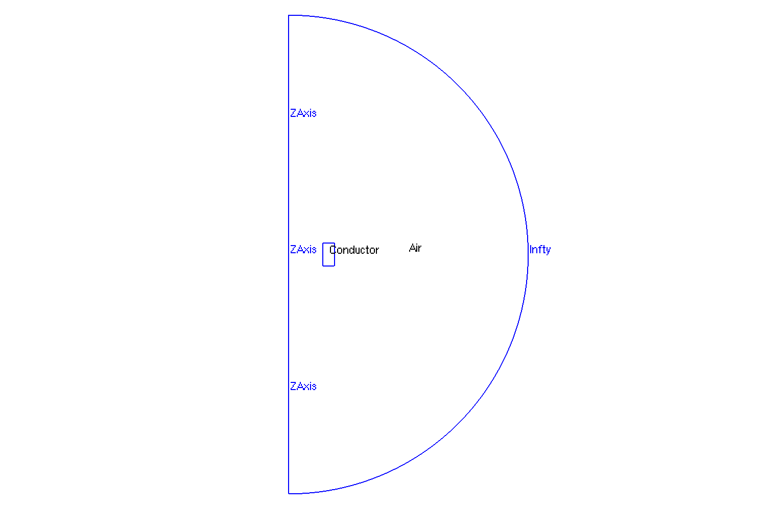
Geometry in Axisymmetrical cut

The geometrical domains are :

Conductor : the torus is composed by conductor material
- Interior : interior surface of conductor ring
- Exterior : exterior surface of conductor ring
- Upper : upper of conductor ring
- Bottom : bottom of conductor ring
Air : the air surround Conductor
- zAxis : a bound of Air, correspond to \(Oz\) axis (\(\{(z,r), \, z=0 \}\))
- infty : the rest of bound of Air

Symbol

Description

value

unit

\(r_{int}\)

interior radius of torus

\(75e-3\)

\(r_{ext}\)

exterior radius of torus

\(100.2e-3\)

\(z_1\)

half-height of torus

\(300e-3\)

\(r_{infty}\)

radius of infty border

\(5*r_{ext}\)

6. Boundary Conditions

We impose the boundary conditions :

Magnetic Equation :
- Strong Dirichlet :
  - On zAxis : \(\Phi = 0\) (\(A_{\theta} = 0\) by symmetric argument)
  - On infty : \(\Phi = 0\) (\(A_{\theta} = 0\) we consider the bound of resolution like infty for magnetic field)
Heat Equation :
- Neumann : \(\frac{\partial T}{\partial \mathbf{n}} = 0\) on Interior and Exterior
- Robin : \(-k \, \frac{\partial T}{\partial \mathbf{n}} = h \, \left( T - T_c \right)\) on Upper and Bottom. The Robin condition represents the cooling by water.
Elastic Equation :
- Strong Dirichlet : \(\mathbf{u} = 0\) on Upper and Bottom. The Dirichlet condition represents the embedding of the mechanical part.
- Neumann : \(\bar{\bar{\sigma}} \cdot \mathbf{n} = 0\) on Interior and Exterior. The Neumann condition represents the freedom of displacement.

On JSON file, the boundary conditions are written :

Boundary conditions on JSON file

    "BoundaryConditions":
    {
        "magnetic":
        {
            "Dirichlet":
            {
                "magdir":
                {
                    "markers":["ZAxis","Infty"],
                    "expr":"0"
                }
            }
        },
        "heat":
        {
            "Robin":
            {
                "heatdir":
                {
                    "markers":["Interior","Exterior"],
                    "expr1":"h*x:h:x",
                    "expr2":"h*T_c*x:h:T_c:x"
                }
            }
        },
        "elastic1":
        {
            "Dirichlet":
            {
                "elasdir":
                {
                    "markers":["Upper","Bottom"],
                    "expr":"{0,0}"
                }
            }
        }
    }

7. Weak Formulation

We obtain :

Weak Formulation of Elastic Thermic Electromagnetism equations in Axisymmetric and Stationnary Case Vectorial

\[\tiny{ \text{(Weak Thermo-Mag Axis Trasnsient)} \\ \left\{ \begin{eqnarray*} \int_{\Omega_c^{axis}}\sigma\frac{\partial \Phi}{\partial t}\cdot \mathbf{ϕ} \ r \ drdz + \int_{\Omega^{axis}}{ \frac{1}{\mu} \tilde{\nabla} \Phi \cdot \tilde{\nabla} \mathbf{ϕ} \ r \ drdz } + \int_{\Omega^{axis}}{\frac{2}{\mu \, r} \frac{\partial \Phi}{\partial r} \, \mathbf{ϕ} \ r \ drdz} = - \int_{\Omega_c^{axis}}{ \sigma \frac{\partial V}{\partial \theta} \mathbf{ϕ} \ r \ drdz } & \text{(Weak AV Axis)} \\ \int_{\Omega_c^{axis}}\rho Cp \frac{\partial T}{\partial t}\mathbf{ϕ} \, r \, drdz +\int_{\Omega_c^{axis}}{ k \, \tilde{\nabla} T \cdot \tilde{\nabla} \mathbf{ϕ} \, r \, drdz } + \int_{\Gamma_R^{axis}}{ h \, T \, \mathbf{ϕ} \, r \, d\Gamma } = \int_{\Omega_c^{axis}}{ Q \, \mathbf{ϕ} \, r \, drdz } + \int_{\Gamma_R^{axis}}{ h \, T_c \, \mathbf{ϕ} \, r \, d\Gamma } & \text{(Weak Heat Axis)} \\ \int_{\Omega_c^{axis}} \frac{\partial^2 u}{\partial t^2}\xi r dr dz\int_{\Omega_c^{axis}} \left( r \left( \lambda \left( \frac{\partial u_r}{\partial r} + \frac{1}{r} u_r + \frac{\partial u_z}{\partial z} \right) - (3\lambda + 2 \mu) \, \alpha_T \, \left( T-T_0 \right) \right) \left( \frac{\partial \xi_r}{\partial r} + \frac{1}{r} \xi_r \right) + r \mu \left[ 2 \left( \frac{\partial u_r}{\partial r} \frac{\partial \xi_r}{\partial r} + \frac{1}{r^2} u_r \xi_r \right) + \left( \frac{\partial u_r}{\partial z} \frac{\partial \xi_r}{\partial z} + \frac{\partial u_z}{\partial r} \frac{\partial \xi_r}{\partial z} \right) \right] \right. \\ \left. + r \mu \left( \frac{\partial u_r}{\partial z} + \frac{\partial u_z}{\partial r} \right) \frac{\partial \xi_z}{\partial r} + r \left[ \lambda \left( \frac{\partial u_r}{\partial r} + \frac{1}{r} u_r + \frac{\partial u_z}{\partial z} \right) + 2\mu \frac{\partial u_z}{\partial z} - (3\lambda + 2 \mu) \, \alpha_T \, \left( T-T_0 \right) \right] \frac{\partial \xi_z}{\partial z} \right) dr dz \\ = \int_{\Omega_c^{axis}}{r \, \mathbf{F}_{laplace} \cdot \mathbf{ξ} \ dr dz} + \int_{\Gamma_{N \hspace{0.05cm} elas}^{axis}}{ r \, \mathbf{g} \cdot \mathbf{ξ} \ dr dz } + \int_{\Gamma_{R \hspace{0.05cm} elas}^{axis}}{ r \left( \mathbf{g} - k \mathbf{u} \right) \cdot \mathbf{ξ} \ dr dz } & \hspace{0.5cm} \text{(Weak Static Elasticity Axis)} \\ \text{for } \mathbf{ϕ} \in H^1(\Omega)^2, \ \psi \in H^1(\Omega_c) , \ \eta \in H^1(\Omega_c), \ \mathbf{ξ} = \begin{pmatrix} xi_x \\ \xi_y \\ \xi_z \end{pmatrix} \in H^1(\Omega_c)^2 \ \text{and} \ \mathbf{F}_{laplace} = \begin{pmatrix} F_{laplace \, r} \\ 0 \\ F_{laplace \, z} \end{pmatrix} = \begin{pmatrix} - \frac{\sigma}{r^2} \frac{\partial V_{\theta}}{\partial \theta} \frac{\partial \Phi}{\partial r} \\ 0 \\ - \frac{\sigma}{r^2} \frac{\partial V_{\theta}}{\partial \theta} \frac{\partial \Phi}{\partial z} \end{pmatrix}_{cyl} \end{eqnarray*} \right. }\]

8. Parameters

The parameters of problem are :

On Conductor :

Symbol

Description

Value

Unit

\(V\)

scalar electrical potential

\( U \, \frac{\theta}{2\pi}\)

\(Volt\)

\(U\)

electrical potential

\(0.2\)

\(Volt\)

\(\sigma\)

electrical conductivity at \(T=T_0\)

\(58e6\)

\(S/m\)

\(j_{\theta}\)

orthoradial current density

\(- \sigma \frac{U}{2\pi} \, \frac{1}{r}\)

\(A/m^2\)

\(\rho\)

density

\(10000\)

\(kg/m^3\)

\(Cp\)

thermal capacity

\(380\)

\(J/K/kg\)

\(E\)

Young Modulus

\(2.1e6\)

\(Pa\)

\(\nu\)

Poisson’s coefficient

\(0.33\)

\(dimensionless\)

\(\lambda\)

Lame’s coefficient

\(\frac{E \, v}{(1-2v)(1+v)}\)

\(Pa\)

\(\mu\)

Lame’s coefficient

\(\frac{E}{2 (1+v)}\)

\(Pa\)

On Air :

Symbol

Description

Value

Unit

\(\mu=\mu_0\)

magnetic permeability of vacuum

\(4\pi.10^{-7}\)

\(kg \, m / A^2 / S^2\)

On JSON file, the parameters are written :

Parameters on JSON file

   "Parameters":
    {
        "bool_laplace":1,
        "bool_dilatation":1,

        "h":80000,
        "T_c":293,
        "T0":293,

        "mu0":"4*pi*1e-7"


    },
    "Materials":
    {
        "Conductor":
        {

            "U":"0.2*t +(-0.2*t+0.2)*(t>1):t",
            "sigma":58e+6,
            "mu":"4*pi*1e-7",

            "k":380,
            "rho":10000,
            "Cp":380,
            "alpha_T":17e-6,

            "E":2.1e6,
            "nu":0.33,

            "j_th":"-sigma*U/2/pi/x:sigma:U:x",

            "Lame_lambda":"E*nu/(1-2*nu)/(1+nu):E:nu",
            "Lame_mu":"E/(2*(1+nu)):E:nu",

            "F_laplace":"{1/x*j_th*(magnetic_grad_Atheta_0*x+magnetic_Atheta),j_th*magnetic_grad_Atheta_1}:x:j_th:magnetic_Atheta:magnetic_grad_Atheta_0:magnetic_grad_Atheta_1",
            "stress_T":"-(3*Lame_lambda+2*Lame_mu)*alphaT*(heat_T-T0):Lame_lambda:Lame_mu:alphaT:heat_T:T0",

            "stress_rr":"(Lame_lambda+2*Lame_mu)*elastic1_grad_u_00+Lame_lambda/x*elastic1_u_0+Lame_lambda*elastic1_grad_u_11+bool_dilatation*stress_T:x:Lame_lambda:Lame_mu:elastic1_u_0:elastic1_grad_u_00:elastic1_grad_u_11:bool_dilatation:stress_T",
            "stress_thth":"Lame_lambda*elastic1_grad_u_00+(Lame_lambda+2*Lame_mu)/x*elastic1_u_0+Lame_lambda*elastic1_grad_u_11+bool_dilatation*stress_T:x:Lame_lambda:Lame_mu:elastic1_u_0:elastic1_grad_u_00:elastic1_grad_u_11:bool_dilatation:stress_T",
            "stress_zz":"Lame_lambda*elastic1_grad_u_00+Lame_lambda/x*elastic1_u_0+(Lame_lambda+2*Lame_mu)*elastic1_grad_u_11+bool_dilatation*stress_T:x:Lame_lambda:Lame_mu:elastic1_u_0:elastic1_grad_u_00:elastic1_grad_u_11:bool_dilatation:stress_T",
            "stress_rz":"Lame_mu*(elastic1_grad_u_01+elastic1_grad_u_10):Lame_mu:elastic1_grad_u_01:elastic1_grad_u_10",

            "stress1":"1/2.*(stress_rr + stress_rz) +sqrt((stress_rr-stress_zz)*(stress_rr-stress_zz)+4*stress_rz*stress_rz):stress_rr:stress_zz:stress_rz",
            "stress2":"stress_thth:stress_thth",
            "stress3":"1/2.*(stress_rr + stress_rz) -sqrt((stress_rr-stress_zz)*(stress_rr-stress_zz)+4*stress_rz*stress_rz):stress_rr:stress_zz:stress_rz"
        },
        "Air":
        {

        }
    },

9. Coefficient Form PDEs

We use the application Coefficient Form PDEs. The coefficient associate to Weak Formulation are :

For MQS equation (Weak MQS Axis) :

On Conductor :

Coefficient

Description

Expression

\(d\)

damping or mass coefficient

\(\sigma\)

\(c\)

diffusion coefficient

\(\frac{r}{\mu}\)

\(\beta\)

convection coefficient

\(\begin{pmatrix} \frac{2}{\mu} \\ 0 \end{pmatrix}\)

\(f\)

source term

\(j_{\theta} \, r^2\)

On Air :

Coefficient

Description

Expression

\(c\)

diffusion coefficient

\(\frac{r}{\mu}\)

\(\beta\)

convection coefficient

\(\begin{pmatrix} \frac{2}{\mu} \\ 0 \end{pmatrix}\)

On JSON file, the coefficients are written :

CFPDEs coefficients on JSON file

   "magnetic":{
        "common":{
            "setup":{
                "unknown":
                {
                    "basis":"Pch1",
                    "name":"Atheta",
                    "symbol":"Atheta"
                }
            }
        },
        "models":[
            {
                "name":"magnetic_Air",
                "materials":"Air",
                "setup":{
                    "coefficients":{
                        "c":"x/mu0:x:mu0",
                        "a":"1/mu0/x:x:mu0"
                    }
                }
            },
            {
                "name":"magnetic_Conductor",
                "materials":"Conductor",
                "setup":{
                    "coefficients":{
                        "c":"x/materials_Conductor_mu:x:materials_Conductor_mu",
                        "a":"1/materials_Conductor_mu/x:x:materials_Conductor_mu",
                        "f":"materials_Conductor_j_th*x:materials_Conductor_j_th:x",
                        "d":"materials_Conductor_sigma*x:x:materials_Conductor_sigma"
                    }
                }
            }
        ]
    },

For heat equation, on Conductor (the temperature isn’t computed on Air)

Coefficient

Description

Expression

\(d\)

damping or mass coefficient

\(\rho \, C_p\)

\(c\)

diffusion coefficient

\(k\)

\(f\)

source term

\(- \sigma \left( \frac{U}{2\pi \, r} +\frac{\partial \Phi}{\partial t}\right)^2\)

On JSON file, the coefficients are written :

CFPDEs coefficients on JSON file

   "heat":{
        "common":{
            "setup":{
                "unknown":
                {
                    "basis":"Pch1",
                    "name":"temperature",
                    "symbol":"T"
                }
            }
        },
        "models":[
            {
                "name":"heat_Conductor",
                "materials":"Conductor",
                "setup":{
                    "coefficients":{
                        "c":"materials_Conductor_k*x:materials_Conductor_k:x",
                        "f":"materials_Conductor_sigma*materials_Conductor_U/(2*pi)*materials_Conductor_U/(2*pi)/x:materials_Conductor_sigma:materials_Conductor_U:x",
                        "d":"materials_Conductor_rho*materials_Conductor_Cp*x:materials_Conductor_rho:materials_Conductor_Cp:x"
                    }
                }
            }
        ]
    },

For elastic equations, on Conductor (the displacement and momentum aren’t computed on Air) :

Displacement (elastic1) :

Coefficient

Description

Expression

\(d\)

damping or mass coefficient

\(r \rho \)

\(f\)

source term

\(\begin{pmatrix} r p_r \\ r p_z \end{pmatrix}\)

Momentum (elastic2) :

Coefficient

Description

Expression

\(\gamma\)

conservative flux source term

\(\begin{pmatrix}-r(\lambda+2\mu)\frac{\partial u_r}{\partial r}-\lambda u_r -r\lambda\frac{\partial u_z}{\partial z} & -r\mu(\frac{\partial u_r}{\partial z}\frac{\partial u_z}{\partial r})\\ -r\mu(\frac{\partial u_r}{\partial z}\frac{\partial u_z}{\partial r}) & -r\lambda\frac{\partial u_r}{\partial r}-\lambda u_r -r(\lambda+2\mu)\frac{\partial u_z}{\partial z} \end{pmatrix}\)

\(f\)

source term

\(\begin{pmatrix} r F_r - \lambda \frac{\partial u_r}{\partial r} - (\lambda+2\mu) \frac{u_r}{r} - \lambda \frac{\partial u_z}{\partial z} \\ r F_z \end{pmatrix}\)

On JSON file, the coefficients are written :

CFPDEs coefficients on JSON file

   "elastic1":{
        "common":{
            "setup":{
                "unknown":
                {
                    "basis":"Pchv1",
                    "name":"displacement",
                    "symbol":"u"
                }
            }
        },
        "models":[
            {
                "name":"elastic1_Conductor",
                "materials":"Conductor",
                "setup":{
                    "coefficients":{
                        "d":"materials_Conductor_rho*x:materials_Conductor_rho:x",
                        "f":"{x*elastic2_v_0,x*elastic2_v_1}:x:elastic2_v_0:elastic2_v_1"
                    }
                }
            }
        ]
    },
    "elastic2":{
        "common":{
            "setup":{
                "unknown":
                {
                    "basis":"Pchv1",
                    "name":"speed",
                    "symbol":"v"
                }
            }
        },
        "models":[
            {
                "name":"elastic2_Conductor",
                "materials":"Conductor",
                "setup":{
                    "coefficients":{
                        "d":"x:x",
                        "gamma":"{-materials_Conductor_stress_rr*x,-materials_Conductor_stress_rz*x,- materials_Conductor_stress_rz*x, -materials_Conductor_stress_zz*x}:x:materials_Conductor_stress_rr:materials_Conductor_stress_rz:materials_Conductor_stress_zz",
                        "f":"{bool_laplace*x*materials_Conductor_F_laplace_0 - materials_Conductor_stress_thth,bool_laplace*x*materials_Conductor_F_laplace_1}:x:bool_laplace:materials_Conductor_F_laplace_0:materials_Conductor_stress_thth:materials_Conductor_F_laplace_1"
                    }
                }
            }
        ]
    }

10. Mesh

Mesh

11. Result

11.1. Displacements

\(u_r(m)\)

\(u_z(m)\)

The radial displacement \(u_r\) is maximum on Or axis in the middle of the torus and decreases to zeros on Upper and Bottom.

The z-displacement is symmetric by Or axis. It is positive on the part and negative on the upper part on the interior side and negative on the part and positive on the upper part on the exterior side.

11.2. Tensor of Deformation \(\bar{\bar{\epsilon}}\)

\(\bar{\bar{\epsilon}}_{rr} = \frac{\partial u_r}{\partial z}\)

\(\bar{\bar{\epsilon}}_{\theta \theta} = \frac{1}{r} \, u_r\)

\(\bar{\bar{\epsilon}}_{zz} = \frac{\partial u_z}{\partial z}\)

\(\bar{\bar{\epsilon}}_{rz} = \frac{1}{2} \left( \frac{\partial u_r}{\partial z} + \frac{\partial u_z}{\partial r} \right)\)

The r-deformation is uniform by z. It is maximal on the middle radius.

The theta-deformation is maximal in Or axis near the interior of the torus and decrease to negative near Upper and Bottom.

The z-deformation is symmetric by the Or axis in the middle of the torus.

The rz-shear is positive on Upper and negative on Bottom.

11.3. Stress Tensor \(\bar{\bar{\sigma}}\)

\(\scriptsize{\bar{\bar{\sigma}}_{rr} = \frac{\lambda}{r} \, u_r + \left( \lambda + 2\mu \right) \, \frac{\partial u_r}{\partial r} + \lambda \, \frac{\partial u_z}{\partial z} - (3\lambda + 2\mu) \, \alpha_T \, \left(T-T_0\right) (Pa)}\)

\(\scriptsize{\bar{\bar{\sigma}}_{\theta \theta} = \frac{\lambda + 2\mu}{r} \, u_r + \lambda \, \frac{\partial u_r}{\partial r} + \lambda \, \frac{\partial u_z}{\partial z}- (3\lambda + 2\mu) \, \alpha_T \, \left(T-T_0\right) (Pa)}\)

\(\scriptsize{\bar{\bar{\sigma}}_{zz} = \frac{\lambda}{r} \, u_r + \lambda \, \frac{\partial u_r}{\partial r} + \left( \lambda + 2\mu \right) \, \frac{\partial u_z}{\partial z} - (3\lambda + 2\mu) \, \alpha_T \, \left( T-T_0 \right) (Pa)}\)

\(\bar{\bar{\sigma}}_{rz} = \mu \, \left( \frac{\partial u_r}{\partial z} + \frac{\partial u_z}{\partial r} \right) (Pa)\)

The radial stress is uniform by the Oz axis and the minimum is reached in the middle.

The orthoradial stress is uniform by the Or axis and the minimum is also reached in the middle.

The z-deformation near of the center is symmetric by Or axis.

The rz-shear is positive on Upper and negative on Bottom.

11.4. Other Tensor

11.4.1. Criterion of Von Mises \(\bar{\bar{\sigma}}_{vm}\)

The tensor of Von Mises permits to say if the matters is in elastic state or not. If the tensor exceeds an matter’s parameter, the matter pass to elastic state to plastic state.

\[\begin{eqnarray*} \bar{\bar{\sigma}}_{Von \, Misses} &=& \sqrt{3 \, J_2} \\ &=& \sqrt{ \frac{13}{2} \, \left( \bar{\bar{\sigma}}_1^2+\bar{\bar{\sigma}}_2^2+\bar{\bar{\sigma}}_3^2-\bar{\bar{\sigma}}_1 \bar{\bar{\sigma}}_2 - \bar{\bar{\sigma}}_1 \bar{\bar{\sigma}}_3 - \bar{\bar{\sigma}}_2 \bar{\bar{\sigma}}_3 \right) } \end{eqnarray*}\]

The \(\sigma_i\) are the principles tensors, the eigenvalues of stress tensor \(\bar{\bar{\sigma}}\).

\(\bar{\bar{\sigma}}_{vm} (Pa)\)

12. References

Elasticity adn toolbox Coefficient Form PDEs, Céline Van Landeghem, 2021, unpublished, Download the PDF

Coupled modelling and simulation of electromagnets in stationnary and instationnary modes (axisymmetric and 3D), J. Nadarasa, June 2 2015, unpublished, page 20-24.

Theorical Physics Reference, Ondřej Čertík, November 29 2011, page 85-90.