Fit & AIR_OUT

In the previous case, we imposed \(A_\theta=0\) on the border infty, which gives results that are not so good near this border. The problem comes for the fact that the analytical solution for \(A_\theta\) on infty is not exactly 0. In order to overcome this problem, we wil implement two methods : fit and AIR_OUT.

1. AIR_OUT

The first method will be to add another layer of Air around the pre-existing air surrounding the conductor. The infty border is pushed back far from the place where we stop our mesurations.

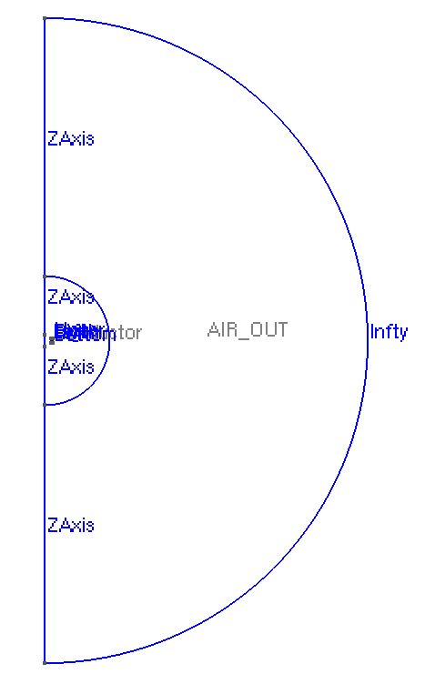
Geometry with AIR_OUT

The Air domain contains the previous Air plus AIR_OUT. The AIR_OUT external border becomes the infty border.

Symbol

Description

value

unit

\(r_{int}\)

interior radius of torus

\(75e-3\)

\(r_{ext}\)

exterior radius of torus

\(100.2e-3\)

\(z_1\)

half-height of torus

\(25e-3\)

\(r_{infty2}\)

radius of infty border

\(5*(5*r_{ext})\)

Mesh size :

Interior of torus : \(0.001 m\)
Far from torus : \(0.004 m\)
Far in AIR_OUT : \(1 m\)

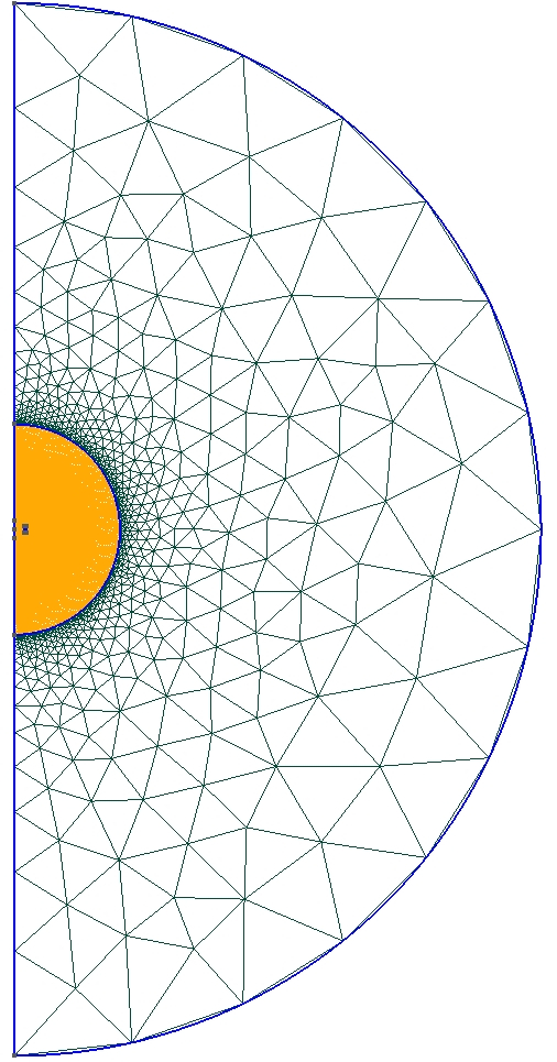
Mesh of Geometry

1.1. Run the Calculation

To run this case, the first thing to do is to change the Meshes reference to 1torus-axis2.geo in the JSON FILE - Edit the file :

    "Meshes":
    {
        "cfpdes":
        {
            "Import":
            {
                "filename":"$cfgdir/1torus-axis2.geo"
            }
        }
    },

The command line to run this case is :

    mpirun -np 16 feelpp_toolbox_coefficientformpdes --config-file=magnetostatic.cfg --cfpdes.gmsh.hsize=1e-3

1.2. Results

We compare this method with the original case :

1.3. Magnetic Potential Field

Table 1. L2 Relative Error Norm for \(A_\theta\) on \(O_r\)
h	Without AIR_OUT	With AIR_OUT
\(9e-3\)	\(2.04\%\)	\(1.38\%\)
\(5e-3\)	\(1.87\%\)	\(1.10\%\)
\(1e-3\)	\(1.80\%\)	\(0.03\%\)
\(5e-4\)	\(1.80\%\)	\(0.02\%\)

Plotting \(\frac{|A^{analytic}-A^{calculated}|}{|A^{analytic}|}\) on \(O_r\) :

1.4. Magnetic Field

Table 2. L2 Relative Error Norm for \(B_z\) on \(O_z\)
h	Without AIR_OUT	With AIR_OUT
\(9e-3\)	\(2.12\%\)	\(2.09\%\)
\(5e-3\)	\(1.06\%\)	\(1.00\%\)
\(1e-3\)	\(0.42\%\)	\(0.13\%\)
\(5e-4\)	\(0.41\%\)	\(0.05\%\)

Plotting \(\frac{|B_z^{analytic}-B_z^{calculated}|}{|B_z^{analytic}|}\) on \(O_z\) :

2. Fit

The second method consit of imposing the analytic solutions of \(A_\theta\) on the border infty. But in order to simplify this process, we will not use a circular arc for the border but 3 sides of a rectangle :

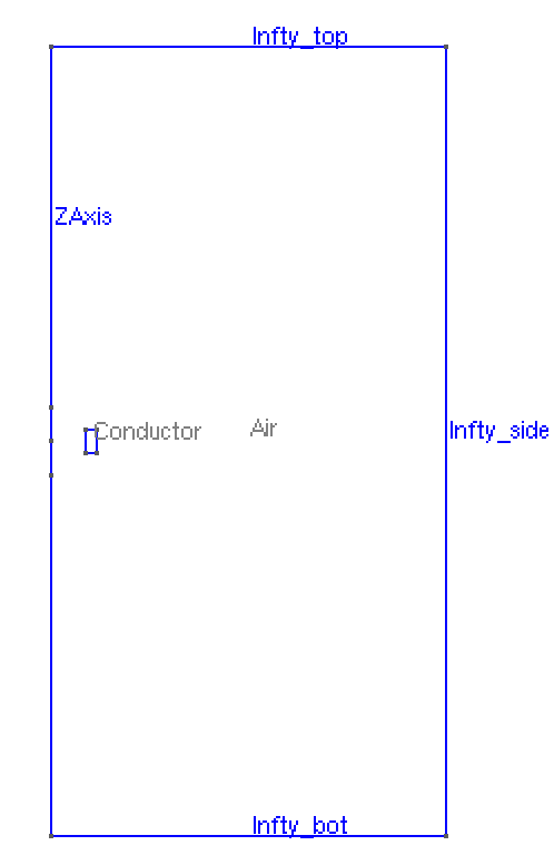
Geometry for the torus with fits

The border Infty is now separated in 3 borders :

Infty_top : the top border of the Air dependent of \(r\)
Infty_bot : the bottom border of the Air dependent of \(r\)
Infty_side : the right border of the Air dependent of \(z\)

Symbol

Description

value

unit

\(r_{int}\)

interior radius of torus

\(75e-3\)

\(r_{ext}\)

exterior radius of torus

\(100.2e-3\)

\(z_1\)

half-height of torus

\(25e-3\)

\(r_{infty}\)

radius of infty border

\(5*r_{ext}\)

Mesh size :

Interior of torus : \(0.001 m\)
Far from torus : \(0.004 m\)

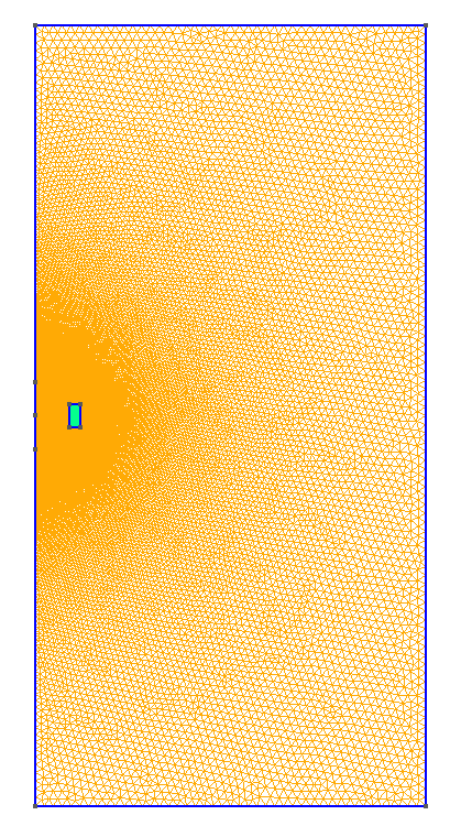
Mesh of Geometry

2.1. Run the Calculation

The command line to run this case is :

    mpirun -np 16 feelpp_toolbox_coefficientformpdes --config-file=magnetostatic_fit.cfg --cfpdes.gmsh.hsize=1e-3

2.2. Data Files

The case data files are available in Github here :

CFG file - Edit the file
JSON file - Edit the file
GEO file - Edit the file

2.3. Parameters

In order to impose the analytical solutions on the borders, we need to use the method "fit" for each subsection of the Infty border.

We give three csv files containing the calculated analytical solutions for each subsection depending on \(r\) for Infty_top and Infty_bot and \(z\) for Infty_side.

On JSON file, the parameters are written :

Parameters on JSON file

    "Parameters":
    {
	    //[...]
        "fit_top": {
            "type":"fit",
            "filename":"$cfgdir/fittop.csv",
            "abscissa":"x",
            "ordinate":"Atheta",
            "interpolation":"P1",
            "expr":"x:x"
          },
        "fit_bot": {
            "type":"fit",
            "filename":"$cfgdir/fitbottom.csv",
            "abscissa":"x",
            "ordinate":"Atheta",
            "interpolation":"P1",
            "expr":"x:x"
          },
        "fit_side": {
            "type":"fit",
            "filename":"$cfgdir/fitside.csv",
            "abscissa":"y",
            "ordinate":"Atheta",
            "interpolation":"P1",
            "expr":"y:y"
          }
    }

2.4. Boundary Conditions

The Dirichlet boundary conditions imposed are :

On zAxis : \(A_{\theta} = 0\)
On Infty_top : \(A_{\theta} = fit\_top\)
On Infty_bot : \(A_{\theta} = fit\_bot\)
On Infty_side : \(A_{\theta} = fit\_side\)

On JSON file, the boundary conditions are written :

Boundary conditions on JSON file

    "BoundaryConditions":
    {
        "magnetic":
        {
            "Dirichlet":
            {
                "ZAxis":
                {
                    "expr":"0"
                },
                "mybc":
                {
                    "markers":["Infty_top"],
                    "expr":"fit_top:fit_top"
                },
                "mybc2":
                {
                    "markers":["Infty_bot"],
                    "expr":"fit_bot:fit_bot"
                },
                "mybc3":
                {
                    "markers":["Infty_side"],
                    "expr":"fit_side:fit_side"
                }
            }
        }
    },

2.5. Results

We compare this method with the original case :

2.6. Magnetic Potential Field

Table 3. L2 Relative Error Norm for \(A_\theta\) on \(O_r\)
h	Without Fits	With Fits
\(9e-3\)	\(2.04\%\)	\(0.87\%\)
\(5e-3\)	\(1.87\%\)	\(0.32\%\)
\(1e-3\)	\(1.80\%\)	\(0.01\%\)
\(5e-4\)	\(1.80\%\)	\(0.00\%\)

Plotting \(\frac{|A^{analytic}-A^{calculated}|}{|A^{analytic}|}\) on \(O_r\) :

2.7. Magnetic Field

Table 4. L2 Relative Error Norm for \(B_z\) on \(O_z\)
h	Without Fits	With Fits
\(9e-3\)	\(2.12\%\)	\(1.99\%\)
\(5e-3\)	\(1.06\%\)	\(0.98\%\)
\(1e-3\)	\(0.42\%\)	\(0.13\%\)
\(5e-4\)	\(0.41\%\)	\(0.06\%\)

Plotting \(\frac{|B_z^{analytic}-B_z^{calculated}|}{|B_z^{analytic}|}\) on \(O_z\) :

3. Comparison of the two methods

Let’s compare the results of the two methods :

3.1. Magnetic Potential Field

Table 5. L2 Error Norm for \(A_\theta\) on \(O_r\)
h	Without AIR_OUT or Fits	With AIR_OUT	With Fits
\(9e-3\)	\(8.71956e-3\)	\(5.88221e-3\)	\(3.71937e-3\)
\(5e-3\)	\(7.93963e-3\)	\(4.70711e-3\)	\(1.37938e-3\)
\(1e-3\)	\(7.64198e-3\)	\(1.43807e-3\)	\(6.26038e-5\)
\(5e-4\)	\(7.63809e-3\)	\(7.77611e-5\)	\(1.51056e-5\)

Table 6. L2 Relative Error Norm for \(A_\theta\) on \(O_r\)
h	Without AIR_OUT or Fits	With AIR_OUT	With Fits
\(9e-3\)	\(2.04\%\)	\(1.38\%\)	\(0.87\%\)
\(5e-3\)	\(1.87\%\)	\(1.10\%\)	\(0.32\%\)
\(1e-3\)	\(1.80\%\)	\(0.03\%\)	\(0.01\%\)
\(5e-4\)	\(1.80\%\)	\(0.02\%\)	\(0.00\%\)

Plotting \(\frac{|A^{analytic}-A^{calculated}|}{|A^{analytic}|}\) on \(O_r\) :

3.2. Magnetic Field

Table 7. L2 Error Norm for \(B_z\) on \(O_z\)
h	Without AIR_OUT or Fits	With AIR_OUT	With Fits
\(9e-3\)	\(15.462408e-2\)	\(15.281730e-2\)	\(14.544868e-2\)
\(5e-3\)	\(7.717275e-2\)	\(7.331173e-2\)	\(7.142153e-2\)
\(1e-3\)	\(3.074955e-2\)	\(9.307516e-3\)	\(9.598967e-3\)
\(5e-4\)	\(2.982289e-2\)	\(3.810487e-3\)	\(4.290458e-3\)

Table 8. L2 Relative Error Norm for \(B_z\) on \(O_z\)
h	Without AIR_OUT or Fits	With AIR_OUT	With Fits
\(9e-3\)	\(2.12\%\)	\(2.09\%\)	\(1.99\%\)
\(5e-3\)	\(1.06\%\)	\(1.00\%\)	\(0.98\%\)
\(1e-3\)	\(0.42\%\)	\(0.13\%\)	\(0.13\%\)
\(5e-4\)	\(0.41\%\)	\(0.05\%\)	\(0.06\%\)

Plotting \(\frac{|B_z^{analytic}-B_z^{calculated}|}{|B_z^{analytic}|}\) on \(O_z\) :

3.3. Conclusion

At the end, both methods give more precise results. The fit method seems to be the better one, but also the harder to implement because an analytical solution is needed, and it must be calculated on all borders before the simulation. The Air_out method is easier to implement and doesn’t need much preparation.