Modelling Airborne Transmission of COVID-19
Following the emergence and quick transmission of the Covid-19 virus, and knowing this virus is transmitted through virus-carrying respiratory droplets,we need a model for indoors airborne transmission that is quick to implement.In order to create such a model, we make some assumptions:
-
the air in the room follows an advection-diffusion-reaction equation
-
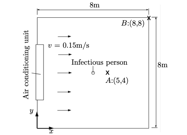
there is only one infectious person in the room
-
the size of the room is \(8m(l)×8m(w)×3m(h)\).
And we test the effect on several ventilation settings:
-
breathing with and without a face mask
-
talking with and without a face mask.
Models studying risk of airborne transmission generally fall into one of two types: the well-mixed room (WMR) assumption and Computational Fluid Dynamics (CFD) models. Well Mixed Room model assume virus-carrying aerosols are evenly dis-tributed throughout the room, so everyone in the room is equally likely to be infected. This assumption greatly simplifies the problem by ignoring the complex effects of the air flow on the airborne particles. These types of models are therefore quick to run, but also too simplistic. Computational Fluid Dynamics simulations are useful in studying airborne transmission as they can take into a count the details of the room size, geometry, the complex turbulent airflow and the size distribution of the aerosols. These models are accurate, but take along time to run and are not suited for «dynamic simulations». Therefore, we develop a model that provides quick simulations and still takes into account turbulence airflow. This model is based on the advection–diffusion–reaction equation.
1. Methodology
We create a 2D model to study the concentration of airborne infectious particles in a rectangular domain. Respiratory droplets are transported via advection due to the airflow in the room and diffusion due to turbulent mixing. We assume the recirculation of air leads to turbulent mixing of the infectious particles. Here is the governing equation for the airborne transmission of COVID-19, the advection–reaction–diffusion equation:
where
-
\(C\) = concentration of airborne infectious particles
-
\(t\) = time
-
\(\nabla\) = two-dimensional gradient operator
-
\(K\) = isotropic eddy diffusion coefficient (turbulent diffusion)
-
\(\vec{x}\) = advection velocity of the air
-
\(S\) = sum of sources and sinks of viral particles.
We model the infected person breathing or talking as a continuous point source emitting viral particles at a constant rate of R particles per second.
Thus, an infectious person talking or breathing at position \((x_0,y_0)\) starting at time \(t=t_0\) is modelled as follows:
where
-
\(\delta(x)\) is the Kronecker delta function
-
\(H(t)\) is the Heaviside step function.
Because R is unknown so far, we assume every respiratory droplets contain the virus and that inhaling and exhaling occur at the same rate. We also assume there is mechanical ventilation in this indoor space provided by air vents.
where \(\lambda\) is the air exchange rate of the room. This is an approximation sincere moval of the air by ventilation occurs at a higher rate near the air vents. Assuming there is only one infectious person, we obtain the following partial differential equation (PDE):
2. Aiflow simulation
In a second time, we will use a more realistic airflow simulation.
2.1. A simplified system for indoor airflow simulation
Even though it is possible to accurately predict some features of airflow within ventilated thanks to advances in computationnal fluid dynamics (CFD) and computer power, it would consume a lot of time to get convergence. Thus, in order to make predictions in short time on a personal computer, we will use a simplified simulation system called «N-point ASOM» (air supply opening model) and developed in 2003 by Bin Zhaoa, Xianting Lib and Qisen Yanb at Tsinghua University, Beijing, China. In 2003, the existing ASOM could be divided into two types:
-
Indirect ones: converting the description of boundary conditions to the description of a box boundary conditions around the supply opening.
-
Direct ones: describing boundary conditions in the vicinity of supply openings. Contrary to indirect methods, they need neither measurements nor empirical formulas. There are mainly two direct ASOMs:
-
Basic model that uses a simple opening with the same effective area as the complex diffuser. It may cause obvious error for a diffuser with small effective area.
-
Momentum model that escribes velocity vectorbased on diffuser effective area. To keep the appropriate supply air mass flow and to introduce the same amount of air into the room, the boundary conditions for continuity equation and momentum equations have to be described separately.
-
In principle, direct ASOM can be applied for any case. Thus, it should be the first choice for engineering application.
«N-point ASOM» combines the positive features of both direct ASOM and momentum method.
2.2. N-point ASOM
The essential of N-point ASOM is to replace the real diffuser by several simple openings so as to reduce thenumber of grids for numerical calculation, while maintaining the inlet momentum and mass flows.
For a supply opening with one discharge direction, the actual inlet momentum flow is
-
\(J_{in}\) = momentum flux (kg.m/s²)
-
\(m\) = mass flow rate (kg/s)
-
\(V_t\) = velocity (m/s)
-
\(L\) = volume flow rate (m³/s)
-
\(A_c\) = effective area of the supply opening (m²)
To describe the right momentum flow while maintainingthe same mass flow rate, the effective area coefficient for calculating the inlet momentum source term in the CFD code is used. That is:
-
\(A\) = gross area of the supply opening (m²)
-
\(R_{fa}\) = ratio of effectivearea to gross area of the supply opening (≤ 1)
| By this equation, inlet momentum flow can be correctly defined and the right inlet mass flow is also given at the same time. It is not necessary to describe boundary conditions formomentum and continuity equations separately. |
The buoyancy inflow of the supply opening is
-
\(g\) = acceleration of gravity (m/s²)
-
\(\Delta\rho\) = difference of supply and indoor air density (kg/m³)
-
\(L\) = supply volume flow rate (m³/s)
For indoor air, we have \(\Delta\rho = -\Delta T\beta\rho,\) \(\beta = \frac{1}{T_0}\) \(\Delta T\) = the difference of supply and indoor air temperature (K) \(\beta\) = volumetric coefficient of expansion (1/K) \(T_0\) = average temperature of indoor air (K)
Therefore,
The \(N\)-point ASOM can ensure \(B\) if \(L\) is correctly defined.
References
-
[covid19-1] Zechariah Lau, Katerina Kaouri, Ian M. Griffiths. Modelling Airborne Transmission of COVID-19 in Indoor Spaces Using anAdvection–Diffusion–Reaction Equation.School of Mathematics, Cardiff University and Mathematical Institute, University of Oxford.
-
[cfd-1] Bin Zhao and Xianting Li. A simplified system for indoor airflow simulation. Building and Environment · April 2003
-
[ibat-www] Zohra Djatouti, Christophe Prud’homme, Vincent Chabannes, Romain Hild IBat Website