COVID-19 transmission
1. Introduction
The COVID-19 pandemic, also known as the coronavirus pandemic, is an ongoing global pandemic of coronavirus disease 2019 (COVID-19), which is caused by severe acute respiratory syndrome coronavirus 2 (SARS-CoV-2). The virus was first identified in December 2019 in Wuhan, China. The World Health Organization declared a Public Health Emergency of International Concern regarding COVID-19 on 30 January 2020, and later declared a pandemic on 11 March 2020. As of 21 August 2021, more than 209 million cases have been confirmed, with more than 4.4 million confirmed deaths attributed to COVID-19, making it one of the deadliest pandemics in history.
Symptoms of COVID-19 are variable, but often include fever, cough, headache, fatigue, breathing difficulties, and loss of smell and taste. Symptoms may begin one to fourteen days after exposure to the virus. At least a third of people who are infected do not develop noticeable symptoms. Of those people who develop noticeable symptoms enough to be classed as patients, most (81%) develop mild to moderate symptoms (up to mild pneumonia), while 14% develop severe symptoms (dyspnea, hypoxia, or more than 50% lung involvement on imaging), and 5% suffer critical symptoms (respiratory failure, shock, or multi-organ dysfunction). Older people are at a higher risk of developing severe symptoms. Some people continue to experience a range of effects (long COVID) for months after recovery, and damage to organs has been observed. Multi-year studies are underway to further investigate the long-term effects of the disease.
Up to now, there is no specific, effective treatment or cure for coronavirus disease. Yet, several experimental treatments are being actively studied in clinical trials.
Several vaccines have also been developed and widely distributed since December 2020 in order to create a herd immunity and avoid the severe virus.
2. Covid-19 transmission modes
The disease caused by the SARS-CoV-2 virus spreads between people in several different ways. It is mainly transmitted via the respiratory route when people inhale droplets and particles that infected people release as they breathe, talk, cough, sneeze, or sing. Infected people are more likely to transmit COVID-19 the longer and closer they interact with others [Wikipedia2021].
On the Figure 1, we illustrate the transmission chain of virus and different modes. When the infected person release the particles they stay suspended in the air or fall on surfaces. Hence, we get infected by breathing the air or touching the contaminated objects when touching the eyes, nose or mouth without cleaning the hands.
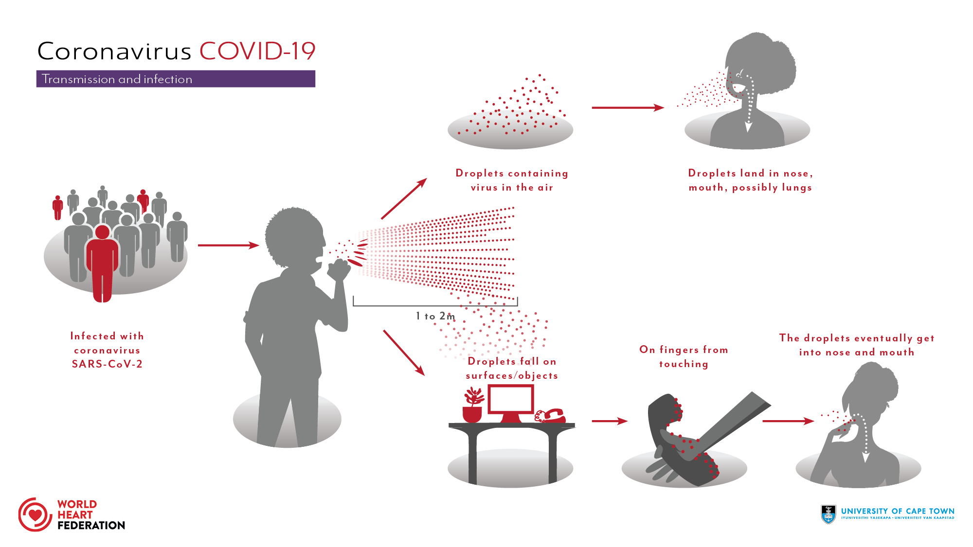
Furthermore, the transmission in indoor spaces is more significant then outdoors. Droplets of various sizes can stay suspended in the air for at least minutes and move across a room. As these droplets are suspended in air they form an aerosol, and transmission via these droplets is called aerosol or airborne transmission.
Current evidence suggests that the virus spreads mainly between people who are in close contact with each other, typically within 1 metre. A person can be infected when aerosols or droplets containing the virus are inhaled or come directly into contact with the eyes, nose, or mouth.
The virus can also spread in poorly ventilated and/or crowded indoor settings, where people tend to spend longer periods of time. This is because aerosols remain suspended in the air or travel farther than 1 metre.
Since the mode of transmission is known, avoiding its spread has been a crucial issue for each country in the world. Many countries have taken recommended preventive measures such as social distancing, wearing face masks, ventilation and air-filtering, hand washing, covering one’s mouth when sneezing or coughing, disinfecting surfaces, self-isolation to isolate their population as much as possible…
3. Interest of modelling COVID-19
As we mentioned, the transmission of COVID-19 virus is a wide issue. Therefor, since its appearance, several model were used to implement the airborne transmission of COVID-19 in indoor spaces which allowed to set up various recommendations. So far, those measures mostly apply to public buildings. Appropriate building engineering controls include sufficient and effective ventilation, possibly enhanced by particle filtration and air disinfection. Ventilation airborne protection measures which already exist can be easily enhanced at a relatively low cost to reduce the number of infections and consequently to save lives.
Ventilation system and COVID-19 transmission
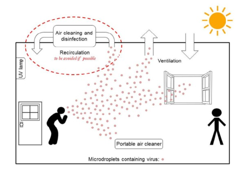
Ventilation is the process of providing outdoor air to a space or building by natural or mechanical means. It controls how quickly room air is removed and replaced over a period of time. Ventilation plays a critical role in removing exhaled virus-laden air, thus lowering the overall concentration and therefore any subsequent dose inhaled by the occupants. Nowadays, the situation can be worse in public buildings and other shared spaces, such as shops, offices, schools, kindergartens, libraries, restaurants, cruise ships, elevators, conference rooms or public transport, where ventilation systems can range from purpose-designed mechanical systems to simply relying on open doors and windows. Hence, in such environments, with lower ventilation rates intended primarily to control indoor air quality, the likelihood of infected persons sharing air with susceptible occupants is high, posing an infection risk contributing to the spread of the infectious disease. As we could notice in the article published by Environment_International [Morawska2020], numerous studies had showed that enhanced ventilation may be a key element in limiting the spread of the SARS-CoV-2 virus. These are the key ventilation-associated recommendations (see Figure 2):
-
to increase the existing ventilation rates and enhance ventilation effectiveness using existing systems.
-
to eliminate any air-recirculation within the ventilation system so as to just supply fresh (outdoor) air.
-
to supplement existing ventilation with portable air cleaners.
-
to avoid over-crowding, e.g. pupils sitting at every other desk in school classrooms, or customers at every other table in restaurants, or every other seat in public transport, cinemas, etc.
However, another work which analysed the effects of the COVID-19 pandemic on thermal comfort and indoor air quality, in winter, in two classrooms of southern Spain with mechanical ventilation systems, has showed that the “emergency” ventilation protocols as a result of the pandemic provide good results in terms of IAQ conditions, but over 60% of teaching hours are in thermal discomfort conditions [Alonso2021].
Other models based for instance on data also showed how progressive restrictions have affected the spread of the epidemic. For example, we consider a model based on Italy’s data [Giordano2020]. Italy has been severely affected by this pandemic and has taken some emergency restrictions as putting on global lockdown several times. The scientists has illustrated the effects of lockdown and population-wide testing. The results showed the importance and effectiveness of a prompt lockdown. However, if the lockdown is weakened, a sudden and strong increase of the spread of disease, a prolonged emergency and more deaths could be expected. Hence, this measure allowed less contracting the virus and avoiding more deaths. Furthermore, they confirm that diagnosis campaigns can reduce the infection peak and help end the epidemic more quickly. The implementation of very strong social-distancing strategies would result in an anticipated lower peak of infected individuals and patients admitted to the Intensive care unit(ICU), with a marked decrease in the total number of infected individuals and ICU admissions due to the disease. All their outputs are also effective for a lot of countries affected by the pandemic.
We can sum up that all those models, implemented since the beginning of the COVID-19 pandemic, had been significantly effective for an easier understanding of the virus transmission, to establish important sanitary measures and also to avoid as mush as possible its spread.
4. Focus on model
By now, we are going to introduce some mathematical models implemented to model airborne transmission of COVID-19. Firstly, we must model the dissemination of the virus in enclosed areas, then the probability of infection.
In this work, we will use a model of ADR equation for the concentration of airborne viral particles indoors which provides rapid predictions. We will also determine the infection risk in the room.
Model based on ADR equation [Lau2021]
We have already introduced the ADR equation and from now on we will apply it to the COVID-19 transmission. Therefore, we introduce a model for the concentration of airborne viral particles indoors, created by [Lau2021].
The authors assumed that:
-
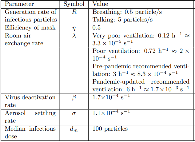
an infectious person talking or breathing with or without a mask who is the source of infectious particles \(S_{inf}\);
-
the room contains an air-conditioning unit;
-
the airborne particles are transported by advection caused by the airflow;
-
the infectious particles are removed due to three factors: the ventilation system, biological deactivation of the virus, and gravitational settling of the virus( \(S_{vent}\), \(S_{deact}\), \(S_{set}\)) .
From these assumptions, they arrived at the advection–diffusion–reaction equation, the governing equation for the concentration of infectious airborne particles:
In the right-hand side of the equation:
-
\(\nabla .( \vec{v}C)\) is the advection term,
-
\(\nabla .(K\nabla C)\) is the diffusion term,
and in the left-side we have the sum of sources and sinks of viral particles.
The coefficients are detailed in Notation and units.
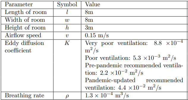
Turbulent diffusion is governed by the eddy diffusion coefficient \(K (m^2/s)\) which is defined by the following formula, valid for an isothermal room served by mixing ventilation:
The Probability of Infection
On the second hand, we are interesting on the infection risk in the room. To simulate the probability of infection, we assume an exponential probability density function of the dose of viral particles inhaled, \(d\). Hence, the probability of infection (infection risk), \(P\), is expressed as
where \(I\) is a constant that depends on the infectiousness of the virus.
To calculate \(d\), the following formula is used:
where \(\rho\) is the average breathing rate.
By substituting this two equations , we obtain the main formula for the probability of infection:
5. Application
In this section, we are going to develop [Lau2021] and our model and explain major modelling assumptions. Subsequently, we will give the values of model parameters.
5.1. Article configuration
First of all, we introduce the modeling framework of the paper [Lau2021]. They assume that:
-
the advection–diffusion–reaction equation governs the concentration of the virus,
-
there is only one infectious person in the room,
-
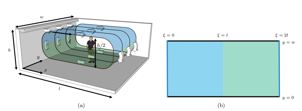
the size of the room is \(8m(l) \times 8m(w) \times 3m(h)\).
The model includes an infected person who is breathing or talking as a continuous point source emitting respiratory particles into the plane of the looping airflow at a constant rate of \(R\) particles/s. They also assume that inhaling and exhaling occur at the same rate, so there is no net source or sink of air from the emitter and receiver of the particles. Thus, an infectious person talking or breathing at position \((\xi_0,y_0)\) is modelled as follows:
where \(\delta(x)\) is the Kronecker delta function.
They assume there is mechanical ventilation in this indoor space provided by air vents. The ventilation effect is modeled as a sink term of uniform strength over the domain,
where \(\lambda\) is the air exchange rate of the room, measured in \(s^{-1}\).
Then, the biological deactivation and gravitational are also settled as particles removal:
where \(\beta\) is the viral deactivation rate and \(\sigma\) is the particle settling rate, all measured in \(s^{-1}\).
Boundary conditions
For a room with length l and width w, they unwrap the loop surface of the airflow to the two-dimensional domain \((\xi, y) \in [0, 2l]\) \(\times [0, w]\)( see Figure 3 (b)). This extended domain allows to model the evolution of the aerosol cloud in both the upper and lower layers of the flow stream in a simpler way. In this setup, the aerosol cloud rejoins the original stream through periodic boundary conditions on the concentration and its derivative at the wall \(\xi =0\) and opposite side of the domain at \(\xi= 2l\):
Moreover, Neumann boundary conditions are applied at the walls located at \(y = 0, w\):
as that no particles pass through the other two walls.
5.2. Our framework
In the second place, we set up our model which we will use to reproduce [Lau2021] results. Therefore, we make the same assumptions that they did and consider the following configuration (see Figure 4).
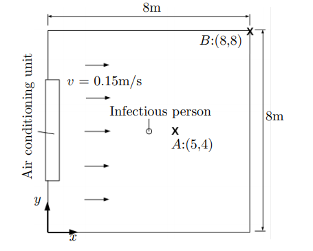
Furthermore, we use the same ADR equation for the concentration of infectious airborne particles and boundary conditions. However, our conditions are for a two dimensional domain \((x, y)\).
Modelling environment and tools
To model the COVID-19 transmission in indoor space, we are going to use a finite library Feel + + which will allow to achieve the simulations. Feel + + is a C + + library for continuous or discontinuous Galerkin methods including finite element method(FEM), spectral element methods(SEM), reduced basis methods, discontinuous Galerkin methods (DG and HDG) in 1D, 2D, 3D and in parallel.
The toolbox used will be Coefficient Form PDEs which provides a general interface for specifying and solving many well-known partial differential equations in the coefficient form. The generic form of PDEs is describe by the next equation:
with \(u\) the unknown and \(\Omega \in R^n\) the computation domain. The coefficients are described in Notation and units. In this equation, we find the same terms involved in our ADR equation:
-
\(\nabla \cdot (-c\nabla u)\) describes diffusion,
-
\(\beta\cdot\nabla u\) describes advection,
-
and finally, \(f\) describes the creation and/or destruction of the quantity.
Firstly, we start by creating the three main files: GEO, CFG and JSON.
We set the room where we study the virus transmission. We create the mesh of our room of size \(8m(l) \times 8m(w) \times 3m(h)\) in the GEO file(see Figure 5).

The CFG (.cfg) files allow to pass command line options to Feel++ applications. In particular, it allows to
-
setup the output directory,
-
setup the mesh,
-
setup the time stepping,
-
define the solution strategy and configure the linear/non-linear algebraic solvers…(see below)
directory=feelpp-project
case.dimension=2

[cfpdes]
filename=$cfgdir/adr.json       #the json file

mesh.filename=$cfgdir/adr.geo   #the geo file
gmsh.hsize=0.05

verbose=0

#solver=Newton
ksp-monitor=1
snes-monitor=1

[cfpdes.equation1]
#time-stepping=Theta
stabilization=1
stabilization.type=supg-pspg

[ts]
time-initial=0
time-step=1             #every second
time-final=14400        #simulations for 240 min
restart.at-last-save=true

[exporter]
freq=1#50#10#20
The JSON (.json) file allows to configure a set of partial differential equations, more precisely it defines :
-
name,
{
    "Name": "Covid-19",      //name we have done to the equation
    "ShortName": "covid19",
-
model,
    "Models":
    {
        "equations":
        [
            {
                "name": "equation1",
                "unknown": {
                    "basis": "Pch1",
                    "name": "solution",
                    "symbol": "C"
                }
            }
        ]
    },
-
parameters,
"Parameters":
    {
        "R": 5,
        "lambda": 3.3e-5,
        "K": 8.8e-4,
        "beta": 1.7e-4,
        "sigma": 1.1e-4,
        "v_x": 0.15,
        "v_y": 0,
        "x_0": 4,
        "y_0": 4,
        "t_0": 0,
        "eps": 0.25,
        "phi": "(t > (t_0-eps))*(t < (t_0+eps)):t:t_0:eps",
        "D": 1
    },
-
materials,
"Materials":
    {
        "mymat1":
        {
            "markers": "Omega",
            "equation1_d": "D:D",
            "equation1_c": "K:K",                    //diffusion
            "equation1_beta": "{v_x, v_y}:v_x:v_y",  //advection
            "equation1_a": " (lambda+ beta+ sigma):lambda:beta:sigma",
            "equation1_f": "(cond*sin(pi*(1+(t-t_0)/eps)/2) + (1-cond)) * R * (1 + cos(pi*sqrt((x-x_0)^2 + (y-y_0)^2)/eps)) / (2 * eps) * (sqrt((x-x_0)^2 + (y-y_0)^2) < eps):t:t_0:eps:cond:R:x_0:y_0:x:y"           //source term
        }
    },
-
initial/boundary conditions,
"BoundaryConditions":
  {
        "equation1":
        {
            "Neumann":
            {
                "mybc1":
                {
                    "markers": "Right",
                    "expr": "v_x*equation1_C:equation1_C:v_x"
                },
                "mybc2":
                {
                    "markers": "Left",
                    "expr": "-v_x*equation1_C:equation1_C:v_x"
                },
                "mybc3":
                {
                    "markers": [ "Bottom","Top" ],
                    "expr": "0"
                }
            }
        }
    },
-
post processing.
"PostProcess":
  {
        "use-model-name": 1,
        "cfpdes":
        {
            "Exports":
            {
                "fields": [ "all" ]
            }
        }
    }
}
Below, the command line we type to launch the simulations which in our case take a few hours on average if we use a powerful machine. It also depends on the time step. The more we take a large step, the more simulation is rapid.
feelpp_toolbox_coefficientformpdes --config-file 2d.cfg
where 2d.cfg is the name of our CFG file.
5.3. Simulation results
After configuring the Feel++ environment, we launch the simulations for 240 minutes. We make the test runs for four different ventilation scenarios:
-
very poor ventilation,
-
poor ventilation,
-
pre-pandemic ventilation,
-
pandemic-updated ventilation.
Thereafter, we visualise the Export.case on Paraview and retrieve the concentration values while positioning at the point \(A\) having coordinates \((5,4)\). Moreover, we extract the concentration values obtained by [Lau2021] to be able to plot them. This figure shows the concentration in the room versus time evaluated at Position \(A\) obtained by the authors of [Lau2021] and us. Position \(A\) is chosen because it is where the highest concentration is while maintaining \(1m\) social distancing from the infectious person. The figure shows that the concentration increases initially, before reaching a steady state. For lower values of \(\lambda\) more time is required to approach the steady-state concentration. At point \(A\), downwind from the source, we can observe that the steady-state concentration is higher for lower values of \(\lambda\), where there is less removal of infectious particles, as expected. Our values for concentration are very close to those obtained by the authors. However, some differences are noticed. It could come from the difference of the room setup.
Thereafter, we use the concentration values to calculate the probability of infection at Position \(A (5,4)\) by using a Python script. The figure above shows the probability of infection versus time evaluated at Position \(A\) for the case of an infectious person just breathing. The figure allows us to compare once again our outputs with those obtained by the authors. We can see on it that the probability of infection growing very slowly initially and becoming more significant with more time spent in the room. Moreover, with pre-pandemic and pandemic updated ventilation, the probability of infection decreases widely. As Position \(A\) is the downwind locations in the room with the highest concentration, it is also the position with the highest infection risk in the room.
References
-
[Ezzati2002] M. Ezzati , DM. Kammen. The health impacts of exposure to indoor air pollution from solid fuels in developing countries: knowledge, gaps, and data needs. Environ. Health Perspect. November 2002. 110 (11): 1057–68.
-
[Jones1999] A.P. Jones, Indoor air quality and health, Atmospheric Environment, Volume 33, Issue 28,1999,Pages 4535-4564,ISSN 1352-2310.
-
[EPA1991] United States, Environmental Protection Agency, Research and Development, Indoor Air Facts No. 4 Sick Building Syndrome,February 1991 .
-
[WHO2010] WHO. New Guidelines for Selected Indoor Chemicals Establish Targets at Which Health Risks are Significantly Reduced,2010.
-
[Singapore1996] Singapore Public Health Ministry of the Environment. Guidelines for Good Indoor Air Quality in Office Premises; Institute of Environmental Epidemiology; Ministry of the Environment: Singapore, 1996; pp. 1–47.
-
[NIOSH2004] NIOSH, NIOSH Pocket Guide to Chemical Hazards, 2004.
-
[Beaulac2020] Vanessa J. Beaulac, Health Canada’s Approach to Indoor Air Contaminants,2020.
-
[Bai2002] Z. Bai, C. Jia, T. Zhu and J. Zhang. Indoor Air Quality Related Standards in China. Proc. Indoor Air 2002, 1012–1017.
-
[MSS2010] Ministère de la santé et des sports, Gestion de la qualité de l’air intérieur, Guide pratique 2010.
-
[HSE2011] Health and Safety Executive. EH40/2005 Workplace Exposure Limits. 2011.
-
[Mannan_Al-Ghambi2021] M. Mannan, S. G. Al-Ghamdi. Indoor Air Quality in Buildings: A Comprehensive Review on the Factors Influencing Air Pollution in Residential and Commercial Structure. Int. J. Environ. Res. Public Health 2021, 18, 3276.
-
[GUO2017] F. Guo. Development of a model for controlling indoor air quality. Earth Sciences. University of Strasbourg, 2017.
-
[Pepper2009] D. W Pepper, D. Carrington. Modeling Indoor Air Pollution,2009.
-
[Kostyrko2020]M. Piasecki, K. Kostyrko. Development of Weighting Scheme for Indoor Air Quality Model Using a Multi-Attribute Decision Making. Energies 2020, 13, 3120.
-
[Wikipedia2021]. Transmission of COVID-19. Wikipedia,2021.
-
[Morawska2020] L. Morawska, J. W. Tang, W. Bahnfleth, P. M. Bluyssen, A. Boerstra, G. Buonanno, J. Cao, S. Dancer, A. Floto, F. Franchimon, C. Haworth, J. Hogeling, C. Isaxon, J. L. Jimenez, J. Kurnitski, Y. Li, M. Loomans, G. Marks, L. C. Marr, L. Mazzarella, A. K. Melikov, S. Miller, D. K. Milton, W. Nazaroff, P. V. Nielsen, C. Noakes, J. Peccia, X. Querol, C. Sekhar, O. Seppänen, S. Tanabe, R. Tellier, K. W. Tham, P. Wargocki, A. Wierzbicka, M. Yao, How can airborne transmission of COVID-19 indoors be minimised?, Environment International,Volume 142,2020,105832,ISSN 0160-4120.
-
[Alonso2021] A. Alonso,J. Llanos, R. Escandón, J.J. Sendra. Effects of the COVID-19 Pandemic on Indoor Air Quality and Thermal Comfort of Primary Schools in Winter in a Mediterranean Climate. Sustainability 2021, 13, 2699.
-
[Giordano2020] G. Giordano, F. Blanchini, R. Bruno, P. Colaneri, A. Di Filippo ,A. Di Matteo and M. Colaneri. Modelling the COVID-19 epidemic and implementation of population-wide interventions in Italy, Nat Med 26, 855–860 (2020).
-
[Lau2021] Z. Lau, K. Kaouri, I. M. Griffiths, A. English. Predicting the Spatially Varying Infection Risk in Indoor Spaces Using an Efficient Airborne Transmission Model, 18th May 2021.
-
[Piasecki2020] Piasecki, Michał & Radziszewska-Zielina, Elżbieta & Czerski, Piotr & Fedorczak-Cisak, Małgorzata & Zielina, Michał & Krzyściak, Paweł & Kwaśniewska-Sip, Patrycja & Grześkowiak, Wojciech. (2020). Implementation of the Indoor Environmental Quality (IEQ) Model for the Assessment of a Retrofitted Historical Masonry Building. Energies. 13. 6051. 10.3390/en13226051.