Perfectly Matched Layer for the Wave Equation

1. Introduction

Acoustic wave propagation in urban environments is a complex and vital field of study with applications spanning urban engineering, environmental acoustics, and urban planning. The ability to predict and analyze sound diffusion in cityscapes is crucial for designing living environments that are both comfortable and compliant with noise regulations. However, accurately modeling the spread of sound waves faces significant challenges due to the diversity of urban structures, the interaction of waves with various obstacles, and the need to simulate extensive open spaces.

Against this backdrop, the adoption of advanced numerical methods such as Perfectly Matched Layers \(\texttt{(PML)}\) has emerged as a solution for absorbing acoustic waves at the computational domain boundaries, thereby simulating a semi-infinite medium without spurious reflections. Originally introduced in the context of \(\texttt{Maxwell}\)'s equations, PMLs have since been adapted and refined for a wide array of wave physics applications.

This report details the development and implementation of a \(\texttt{Feel++}\)-based model for the study of acoustic wave propagation in a urban neighborhood, modeled as a homogenous medium at the scale of a city block. We will delve into the underlying theory of \(\texttt{PMLs}\) and their integration into the acoustic wave equation, with a focus on the non-reflecting conditions of the waves.

Acoustic wave propagation is given by the following equation:

\[\frac{1}{\mu}\frac{\partial^2 p}{\partial t^2} - \nabla \cdot \left( \frac{1}{\rho} \nabla p \right) = \frac{\partial F}{\partial t}\]

For the sake of simplicity, we will introduce the \(\texttt{PMLs}\) to the first-order acoustic system in time:

\[\begin{align*} \frac{1}{\mu}\frac{\partial p}{\partial t} - \nabla \cdot v &= F \qquad \text{ in } \Omega \times (0,T) \\ \rho \frac{\partial v}{\partial t} - \nabla p &= 0 \qquad \text{ in } \Omega \times (0,T) \\ p(x,0) &= 0 \qquad \text{ in } \Omega \\ v(x,0) &= 0 \qquad \text{ in } \Omega \end{align*}\]

where \(p\) is the acoustic pressure, \(v\) is the acoustic velocity, \(\mu\) is the dynamic viscosity, \(\rho\) is the density, and \(F\) is the source term.

Initially, we implement a Perfectly Matched Layer \(\texttt{(PML)}\) formulation that is of order \(d\) in time. Assuming the differentiability of the absorption coefficients, we demonstrate the feasibility of achieving an optimal first-order system in time.

2. Setting up a formulation in PML

We now revisit the PML method that aims at constructing artificial layers (of finite thickness) surrounding the physical bounded domain \(\Omega_{BD}\) and designed in such a way that the incoming waves (entering into the layers) are not reflected at the interface with the physical domain and decay exponentially into them. In the following, we implicitly assume that all the outgoing waves (leaving the physical domain of interest) correspond to purely forward propagating waves in the direction normal to the interface, i.e. there is no backward propagating waves or evanescent waves.

We consider a bounded Cartesian domain \(\Omega_{BD} = [-l_i,l_i ]^d\) surrounded by an artificial absorbing layer (the \(\texttt{PML}\) region) \(\Omega_{PML} = [-l_i - h_i, l_i + h_i ]^d \setminus \Omega_{BD}\) with \(h_i\) the thickness of the \(\texttt{PML}\) layer. The \(\texttt{PML}\) region \(\Omega_{PML}\) is divided into \(d\) subdomains \(\Omega_i\) with \(i = 1, \dots, d\) such that \(\Omega_i = \{x \in \Omega_{PML} ; |x_i| > l_i \}\) and the outgoing propagative waves are attenuated in the \(xi\)-direction within \(\texttt{PML}\) subregions \(\Omega_i\).

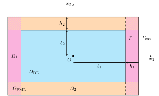
Figure 1. A Illustration of the PML region in 2D

Physical bounded domain \(\Omega_{BD}\) surrounded by an artificial \(\texttt{PML}\) region \(\Omega_{PML} = \cup_{i=1}^d \Omega_i\) divided into \(d\) overlapping subregions \(\Omega_i\) with interface \(\Gamma = \partial\Omega_{BD} \cap \partial\Omega_{PML}\) and exterior boundary \(\Gamma_{ext} = \partial\Omega_{PML} \setminus \Gamma\) .

We denote by \(\Gamma = \partial\Omega_{BD} \cap \partial\Omega_{PML}\) and \(\Gamma_i = \partial\Omega_{BD} \cap \partial\Omega_{i}\) , the interface between the physical domain \(\Omega_{BD}\) and the PML region \(\Omega_{PML}\) (resp. the PML subregion \(\Omega_{i}\)) , and by \(n = n_i e_i\) the unit normal vector to \(\Gamma\) pointing outward \(\Omega_{BD}\) . Furthermore, we define the entire domain \(\Omega = \Omega_{BD} \cup \Omega_{PML}\) as the disjoint union between \(\Omega_{BD}\) and \(\Omega_{PML}\) , and we denote by \(\Gamma_{ext}\) the part of its boundary \(\partial\Omega\) that coincides with the exterior boundary of \(\Omega_{PML}\) , that is \(\Gamma_{ext} = \partial\Omega_{PML} \setminus \Gamma \cup \Gamma_{free}\) , where \(\Gamma_{free}\) stands for the possible free surfaces in the case where a semi-infinite medium with free-surface boundary conditions is considered.

2.1. Complex coordinate stretching

In the frequency domain, the \(\texttt{PML}\) method consists in analytically stretching one or more real spatial coordinate(s) of the physical wave equations into the complex plane \(\mathcal{C}\), the ones corresponding to the direction(s) along which the outwardly propagating waves have to be attenuated in the absorbing layers. In the following, for any complex number \(z \in \mathbb{C}\), we denote by \(\mathcal{R}_e(z)\) and \(\mathcal{I}_m(z)\) the real and imaginary parts of \(z\) respectively.

Following the complex coordinate stretching, we introduce a complex change \(\tilde{x}_j\) defined by:

\[\begin{align*} \tilde{x}_j &= x_j + \frac{i}{\omega} \int_0^{x_j} \tau_j(s) ds \end{align*}\]

where the functions \(\tau_j\) , ranging from 1 to d, are continuous, positive functions that depend only on \(x_j\) and are zero in the physical domain (i.e., for negative \(x_j\) ). In our case, we will further assume that these functions are differentiable and have continuous derivatives (thus zero in the physical domain).

The functions \(\tau_j\) are called absorption coefficients following \(x_j\).

2.2. Implementation steps

For the implementation of the formulation in the \(\texttt{PMLs}\), we will proceed as follows:

Transition to the frequency domain through the application of the Fourier transform in time.
Extension of the equations into the complex space thanks to the new coordinate system \((\tilde{x}_j)_{j=1..d}\).
Introduction of the complex parameter for the reinterpretation of the system in the form of partial differential equations in \((x_j)_{j=1..d}\).
Introduction of new unknowns in order to obtain a system that involves only positive powers of \(-i\omega\), the goal being to reinterpret the obtained system in the form of temporal partial differential equations.
Obtain the system to be solved in \(\texttt{PML}\) by applying the inverse Fourier time Fourier transform to the system obtained in step 4.

2.2.1. Step 1: Transformation to the Frequency Domain

Setting aside the initial conditions and the source function located in the physical domain, we proceed with a transformation to the frequency domain. This yields:

\[\begin{align} -i\omega \frac{1}{\mu} \hat{p} - \nabla \cdot \hat{v} &= 0, \label{eq:3.1} \end{align}\]

\[\begin{align} -i\omega \rho \hat{v} - \nabla \hat{p} &= 0 \label{eq:3.2} \end{align}\]

where \(\hat{p} = \mathcal{F}_t(p)\) and \(\hat{v} = \mathcal{F}_t(v)\), \(\mathcal{F}_t\) representing the Fourier transforms in time.

2.2.2. Step 2: Equation Extension with a New Coordinate System

By extending these equations through a new coordinate system, we arrive at:

\[\begin{align} -i\omega \frac{1}{\mu} \hat{p} - \tilde{\nabla} \cdot \hat{v} &= 0, \label{eq:3.3} \end{align}\]

\[\begin{align} -i\omega \rho \hat{v} &= \tilde{\nabla}\hat{p}, \label{eq:3.4} \end{align}\]

where \(\tilde{\nabla} = \left( \frac{\partial}{\partial \tilde{x}_j} \right)^*_{j=1..d}\).

2.2.3. Step 3: Transformation and Diagonal Matrix

We observe:

\[\begin{align} \frac{\partial}{\partial \tilde{x}_j} &= \frac{i\omega}{i\omega - \tau_j} \frac{\partial}{\partial x_j}, \quad \forall j = 1..d. \label{eq:3.5} \end{align}\]

As a result, \(\nabla\) and \(\tilde{\nabla}\) satisfy \(\nabla = M \tilde{\nabla}\) where \(M\) is a \(d \times d\) diagonal matrix with diagonal elements \(M_{jj} = 1 + \frac{i\tau_j}{\omega}\).

The system is then rewritten as:

\[\begin{align} -i\omega \frac{1}{\mu} \hat{p} - \sum_{k=1}^{d} M_{kk}^{-1} \frac{\partial \hat{v}_k}{\partial x_k} &= 0, \label{eq:3.6} \end{align}\]

\[\begin{align} -i\omega M \rho \hat{v} &= \nabla \hat{p}, \label{eq:3.7} \end{align}\]

with \(\hat{v} = (\hat{v}_k)_{k=1..d}\).

2.2.4. Step 4: Focusing on the Second Term

We shall now turn our attention to the second term of the second equation. Since \(M^{-1}\) depends on \((-i\omega + \tau_{x})^{-1}\), this equation cannot be reinterpreted as a temporal partial differential equation after applying the inverse Fourier transform \(\mathcal{F}^{-1}_t\) to the temporal domain. We then introduce \(\tilde{v}\) such that:

\[\begin{align} M\tilde{v} &= \hat{v}. \label{eq:3.8} \end{align}\]

\(\tilde{v}_k\) satisfies:

\[\begin{align} M_{kk} \tilde{v}_k &= \hat{v}_k. \label{eq:3.9} \end{align}\]

Utilizing the fact that \(M_{kk} = 1 + \frac{i\tau_k}{\omega}\) and considering that the functions \(\tau_k\) depend only on \(x_k\), we derive:

\[\begin{align} \frac{\partial \hat{v}_k}{\partial x_k} &= M_{kk} \frac{\partial \tilde{v}_k}{\partial x_k} + \frac{dM_{kk}}{dx_k} \tilde{v}_k, \label{eq:3.10} \end{align}\]

which simplifies to:

\[\begin{align} M_{kk}^{-1} \frac{\partial \hat{v}_k}{\partial x_k} &= \frac{\partial \tilde{v}_k}{\partial x_k} + M_{kk}^{-1} \frac{dM_{kk}}{dx_k} \tilde{v}_k. \label{eq:3.11} \end{align}\]

Rewriting system, we get:

\[\begin{align} -i\omega \frac{1}{\mu} \hat{p} - \nabla \cdot \tilde{v} - \sum_{k=1}^{d} M_{kk}^{-1} \frac{dM_{kk}}{dx_k}\tilde{v}_k &= 0, \label{eq:3.12} \end{align}\]

\[\begin{align} -i\omega M \rho M \tilde{v} &= \nabla \hat{p}. \label{eq:3.13} \end{align}\]

We introduce new vector unknowns:

\[\begin{align} M \hat{v}^o &= M' \tilde{v}, \label{eq:3.14} \end{align}\]

\[\begin{align} \hat{v}^* &= \rho M \tilde{v}, \label{eq:3.15} \end{align}\]

where \(M'\) is the diagonal matrix of size \(d \times d\) with diagonal elements \(M'_{kk} = \frac{dM_{kk}}{dx_k}\).

Let \(T\) and \(T'\) be two \(d \times d\) diagonal matrices with respective diagonal elements \(T_{kk} = \tau_k\) and \(T'_{kk} = \frac{d\tau_k}{dx_k}\). We establish the equalities:

\[\begin{align} -i\omega M &= -i\omega I_{dd} + T \label{eq:3.16} \end{align}\]

and

\[\begin{align} -i\omega M' &= T'. \label{eq:3.17} \end{align}\]

This allows us to reformulate the system as:

\[\begin{align} -i\omega \frac{1}{\mu}\hat{p} - \nabla \cdot \tilde{v} - \sum_{k=1}^{d} \hat{v}^o \cdot \overrightarrow{e_k} &= 0, \label{eq:3.18} \end{align}\]

\[\begin{align} -i\omega \hat{v}^* + T \hat{v}^* &= \nabla \hat{p}, \label{eq:3.19} \end{align}\]

\[\begin{align} -i\omega \hat{v}^o + T' \hat{v}^o &= T' \tilde{v} \label{eq:3.20} \end{align}\]

\[\begin{align} -i\omega \hat{v}^* &= -i\omega \rho \tilde{v} + \rho T \tilde{v}. \label{eq:3.21} \end{align}\]

where \((\overrightarrow{e_k})_{k=1..d}\) is the canonical basis of \(\mathbb{R}^d\).

2.2.5. Step 5: Inverse Fourier Transform

We extend by continuity the equality \(\tilde{v} = \hat{v}= \mathcal{F}_t(v)\), verified in the physical domain, to all the \(\texttt{PML}\) and obtain \(\mathcal{F}^{-1}(\tilde{v}) = v\) in \(\Omega \cup \Omega_{PML}\). Let us denote \(v^* = \mathcal{F}^{-1}_t(\hat{v}*)\) and \(v^o = \mathcal{F}^{-1}_t(\hat{v}^o)\).

Applying the inverse Fourier transform \(\mathcal{F}^{-1}_t\) to system , we obtain the system to be solved in the \(\texttt{PML}\) to which we introduce Dirichlet boundary conditions on \(p\):

\[\begin{align} \frac{1}{\mu} \frac{\partial p}{\partial t} - \nabla \cdot v - \sum_{k=1}^{d} v^o \cdot \overrightarrow{e_k} &= 0 \quad \text{in} \quad \Omega_{PML}, \\ \frac{\partial v^*}{\partial t} + T v^* &= \nabla p \quad \text{in} \quad \Omega_{PML}, \\ \frac{\partial v^o}{\partial t} + T' v^o &= T' v^o \quad \text{in} \quad \Omega_{PML}, \\ \rho \frac{\partial v}{\partial t} + \rho T v &= \frac{\partial v^*}{\partial t} \quad \text{in} \quad \Omega_{PML},\\ p &= 0 \quad \text{on} \quad \partial\Omega_{PML}. \label{eq:3.26} \end{align}\]

In this formulation, we introduce an additional vector variable, together, these equations define the dynamics of the pressure and velocity fields in PMLs keeping the system of order 1 in time, allowing efficient wave absorption to minimize artificial reflections in numerical simulations.

2.3. Variational Formulation

We now introduce the variational formulation of the system in the \(\texttt{PMLs}\). We multiply the first equation by \(\phi\), the second equation by \(\psi^*\), the third equation by \(\psi^o\), and the fourth equation by \(\psi\) and integrate over the \(\texttt{PML}\) region \(\Omega_{PML}\). With integration by parts and the use of the boundary conditions, we obtain:

Find \((p \in L^2(0,T;H_0^1(\Omega_{PML})))\) and \((v,v^*,v^o \in L^2(0,T;L^2([\Omega_{PML}]^d)))\) such that:

\[\begin{align} \frac{\partial}{\partial t} \int_{\Omega_{PML}} \frac{1}{\mu} p \phi dx + \int_{\Omega_{PML}} v \cdot \nabla \phi dx + \sum_{k=1}^{d} \int_{\Omega_{PML}} v^o \cdot \overrightarrow{e_k} \phi dx &= 0 \quad \forall \phi \in H_0^1(\Omega_{PML}), \end{align}\]

\[\begin{align} \frac{\partial}{\partial t} \int_{\Omega_{PML}} v^* \psi^* dx + \int_{\Omega_{PML}} T v^* \psi^* dx &= \int_{\Omega_{PML}} \nabla p \psi^* dx \quad \forall \psi^* \in L^2([\Omega_{PML}]^d), \end{align}\]

\[\begin{align} \frac{\partial}{\partial t} \int_{\Omega_{PML}} v^o \psi^o dx + \int_{\Omega_{PML}} T' v^o \psi^o dx &= \int_{\Omega_{PML}} T' v^o \psi^o dx \quad \forall \psi^o \in L^2([\Omega_{PML}]^d), \end{align}\]

\[\begin{align} \frac{\partial}{\partial t} \int_{\Omega_{PML}} \rho v \psi dx + \int_{\Omega_{PML}} \rho T v \psi dx &= \int_{\Omega_{PML}} \frac{\partial v^*}{\partial t} \psi dx \quad \forall \psi \in L^2([\Omega_{PML}]^d). \end{align}\]

3. References

[1] Sandrine Fauqueux. Eléments finis mixtes spectraux et couches absorbantes parfaitement adaptées pour la propagation d’ondes élastiques en régime transitoire. Modélisation et simulation. ENSTA ParisTech, 2003. Français. NNT : 2003PA090002. tel-00007445
[2] Florent Pled, Christophe Desceliers. Review and Recent Developments on the Perfectly Matched Layer (PML) Method for the Numerical Modeling and Simulation of Elastic Wave Propagation in Unbounded Domains. Archives of Computational Methods in Engineering, 2022, 10.1007/s11831-021-09581-y. hal-03196974