Wave equation using finite difference

1. Problem statement

We aim to solve the acoustic wave equation in a homogeneous rectangular medium using FDTD. Mathematically, the problem is stated as follows:

\[\begin{cases} \begin{align} \partial_t^2 u(x,y,t) - c^2 \Delta_{xy} u(x,y,t) &= s(x,y,t) \quad (x,y) \in [0,L]\times[0,H], \quad t \in [0,T] \\ u(x,y,0) &= f(x,y) \\ \partial_t u(x,y,0) &= g(x,y) \\ \partial_n u(x,y,t) &= k(x,y,t) \quad (x,y) \in \partial\Omega, \quad t \in [0,T] \end{align} \end{cases}\]

Equation’s parameters are

$u$ is the function to be determined (that describes the wave)
$c$ is the wave velocity (assumed given constant)
$\Delta_{xy}$ is the Laplacian operator in space
$s$ is the source term (assumed given function)
$L$ is the length of the domain (assumed given constant)
$H$ is the height of the domain (assumed given constant)
$T$ is the final time (assumed given constant)
$f$ is the initial condition for $u$ (assumed given function)
$g$ is the initial condition for $\partial_t u$ (assumed given function)
$k$ is the boundary condition for $\partial_n u$ (Neumann condition: assumed given function)
$\partial \Omega$ denotes the boundary of the domain.

1.1. Semi-discretization in space

We use a finite difference scheme to discretize the Laplacian operator in space. Let’s introduce a uniform grid defined by its vertices of coordinates :

\[x_i = i \Delta x, \quad y_j = j \Delta y, \quad t^n = n \Delta t, \quad \text{with } i \in [\![0;I]\!] \quad \text{and} \quad j \in [\![0;J]\!]\]

where $\Delta x = \frac{L}{I}$ and $\Delta y = \frac{H}{J}$ are the space steps, and $\Delta t$ is the time step. We denote by $u_{i,j}(t)$ the approximation of $u(x_i,y_j,t)$ and by $u_{i,j}^n$ the approximation of $u(x_i,y_j,t^n)$.

Figure 1. A Finite difference grid

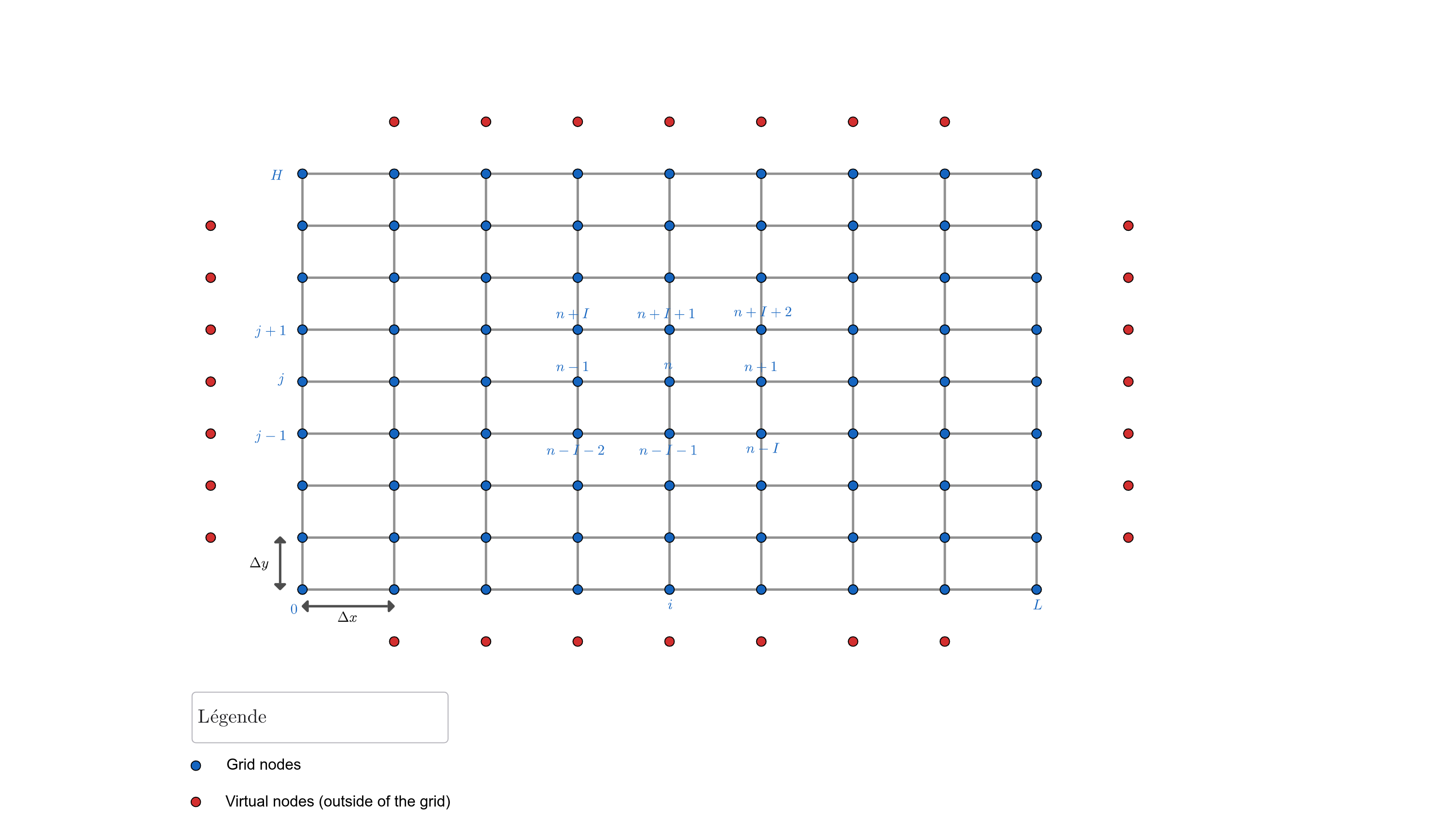
Inside the domain, we approximate the second-order partial derivatives using three-point central differences. At the edges, except at the corners, we approximate the first-order partial derivatives using two-point central differences of second order. For simplicity, at the corners, we approximate the first-order partial derivatives using two-point off-centered differences of first order.

To get $u_{i,j}$ as vector, we define $U_n = u_{i,j}$ with the bijection $n = n(i,j) = i+j(I+1)$. So after discretization, we write all the discretized equations in the form of a linear system of the form $A \tilde U = F$, where

$A$ is a matrix with size $[(I+1)(J+1)]^2$,
$\tilde U = (U_1, U_2, \ldots )$ is the vector of unknowns with size $(I+1)(J+1)$ and
$F$ is the right hand side vector with size $(I+1)(J+1)$.

1.1.1. Inside the domain

Inside the domain, indices $i$ and $j$ vary in $[\![1;I-1]\!]$ and $[\![1;J-1]\!]$ respectively.

By expanding and summing, the discretization can be written as :

\[u''_{i,j}(t) - \frac{c^2}{\Delta y^2} u_{i,j-1}(t) - \frac{c^2}{\Delta x^2} u_{i-1,j}(t) + 2c^2 (\frac{1}{\Delta x^2} + \frac{1}{\Delta y^2}) u_{i,j}(t) - \frac{c^2}{\Delta x^2} u_{i+1,j}(t) - \frac{c^2}{\Delta y^2} u_{i,j+1}(t) = s_{i,j}(t)\]

which is equivalent to :

\[U''_n(t) - \frac{c^2}{\Delta y^2} U_{n-I-1}(t) - \frac{c^2}{\Delta x^2} U_{n-1}(t) + 2c^2 (\frac{1}{\Delta x^2} + \frac{1}{\Delta y^2}) U_n(t) - \frac{c^2}{\Delta x^2} U_{n+1}(t) - \frac{c^2}{\Delta y^2} U_{n+I+1}(t) = S_n(t)\]

where $S_n(t) = s_{i,j}(t)$.

We deduce the matrix $A$ and the vector $F$ as follows:

\[\begin{cases} \begin{align} A_{n,n-I-1} &= A_{n,n+I+1} = -\frac{c^2}{\Delta y^2} \\ A_{n,n-1} &= A_{n,n+1} = -\frac{c^2}{\Delta x^2} \\ A_{n,n} &= 2c^2 (\frac{1}{\Delta x^2} + \frac{1}{\Delta y^2}) \\ F_n(t) &= S_n(t) \end{align} \end{cases}\]

1.1.2. At the edges (except corners)

In order to approximate first-order partial derivatives using two-point central differences of second order, we use the virtual points located outside the domain. After that, we eliminate them, so that they do not appear in the linear system.

At bottom edge

At the bottom edge, indices $i$ vary in $[\![1;I-1]\!]$ and $j=0$.

By expanding and summing, the discretization can be written as :

\[u''_{i,0}(t) - \frac{c^2}{\Delta x^2} u_{i-1,0}(t) + 2c^2(\frac{1}{\Delta x^2} + \frac{1}{\Delta y^2} u_{i,0})(t) - \frac{c^2}{\Delta x^2} u_{i+1,0}(t) - \frac{2c^2}{\Delta y^2} u_{i,1}(t) = s_{i,0}(t) + \frac{2c^2}{\Delta y} k_{i,0}(t)\]

which is equivalent to :

\[U'_n - \frac{c^2}{\Delta x^2} U_{n-1}(t) + 2c^2(\frac{1}{\Delta x^2} + \frac{1}{\Delta y^2}) U_n(t) - \frac{c^2}{\Delta x^2} U_{n+1}(t) - \frac{2c^2}{\Delta y^2} U_{n+I+1}(t) = S_n(t) + \frac{2c^2}{\Delta y} K_n(t)\]

We deduce the matrix $A$ and the vector $F$ as follows:

\[\begin{cases} \begin{align} A_{n,n-1} &= A_{n,n+1} = -\frac{c^2}{\Delta x^2} \\ A_{n,n} &= 2c^2 (\frac{1}{\Delta x^2} + \frac{1}{\Delta y^2}) \\ A_{n,n+I+1} &= -\frac{2c^2}{\Delta y^2} \\ F_n(t) &= S_n(t) + \frac{2c^2}{\Delta y} K_n(t) \end{align} \end{cases}\]

At left edge

At the left edge, indices $i=0$ and $j$ vary in $[\![1;J-1]\!]$.

By expanding and summing, the discretization can be written as :

\[u''_{0,j}(t) - \frac{c^2}{\Delta y^2} u_{0,j-1}(t) - \frac{2c^2}{\Delta x^2} u_{1,j}(t) + 2c^2(\frac{1}{\Delta x^2} + \frac{1}{\Delta y^2} u_{0,j})(t) - \frac{c^2}{\Delta y^2} u_{0,j+1}(t) = s_{0,j}(t) + \frac{2c^2}{\Delta x} k_{0,j}(t)\]

which is equivalent to :

\[U''_n(t) - \frac{c^2}{\Delta y^2} U_{n-I-1}(t) - \frac{2c^2}{\Delta x^2} U_{n+1}(t) + 2c^2(\frac{1}{\Delta x^2} + \frac{1}{\Delta y^2}) U_n(t) - \frac{c^2}{\Delta y^2} U_{n+I+1}(t) = S_n(t) + \frac{2c^2}{\Delta x} K_n(t)\]

We deduce the matrix $A$ and the vector $F$ as follows:

\[\begin{cases} \begin{align} A_{n, n-I-1} &= A_{n,n+I+1} = -\frac{c^2}{\Delta y^2} \\ A_{n,n} &= 2c^2 (\frac{1}{\Delta x^2} + \frac{1}{\Delta y^2}) \\ A_{n,n+1} &= -\frac{2c^2}{\Delta x^2} \\ F_n(t) &= S_n(t) + \frac{2c^2}{\Delta x} K_n(t) \end{align} \end{cases}\]

At top edge

At the top edge, indices $i$ vary in $[\![1;I-1]\!]$ and $j=J$.

By expanding and summing, the discretization can be written as :

\[u''_{i,J}(t) - \frac{c^2}{\Delta x^2} u_{i-1,J}(t) + 2c^2(\frac{1}{\Delta x^2} + \frac{1}{\Delta y^2} u_{i,J})(t) - \frac{c^2}{\Delta x^2} u_{i+1,J}(t) - \frac{2c^2}{\Delta y^2} u_{i,J-1}(t) = s_{i,J}(t) + \frac{2c^2}{\Delta y} k_{i,J}(t)\]

which is equivalent to :

\[U'_n - \frac{c^2}{\Delta x^2} U_{n-1}(t) + 2c^2(\frac{1}{\Delta x^2} + \frac{1}{\Delta y^2}) U_n(t) - \frac{c^2}{\Delta x^2} U_{n+1}(t) - \frac{2c^2}{\Delta y^2} U_{n-I-1}(t) = S_n(t) + \frac{2c^2}{\Delta y} K_n(t)\]

We deduce the matrix $A$ and the vector $F$ as follows:

\[\begin{cases} \begin{align} A_{n,n-1} &= A_{n,n+1} = -\frac{c^2}{\Delta x^2} \\ A_{n,n} &= 2c^2 (\frac{1}{\Delta x^2} + \frac{1}{\Delta y^2}) \\ A_{n,n-I-1} &= -\frac{2c^2}{\Delta y^2} \\ F_n(t) &= S_n(t) + \frac{2c^2}{\Delta y} K_n(t) \end{align} \end{cases}\]

At right edge

At the right edge, indices $i=I$ and $j$ vary in $[\![1;J-1]\!]$.

By expanding and summing, the discretization can be written as :

\[u''_{I,j}(t) - \frac{2c^2}{\Delta x^2} u_{I-1,j}(t) + 2c^2(\frac{1}{\Delta x^2} + \frac{1}{\Delta y^2} u_{I,j})(t) - \frac{c^2}{\Delta y^2} u_{I,j-1}(t) - \frac{c^2}{\Delta y^2} u_{I,j+1}(t) = s_{I,j}(t) + \frac{2c^2}{\Delta x} k_{I,j}(t)\]

which is equivalent to :

\[U''_n(t) - \frac{2c^2}{\Delta x^2} U_{n-1}(t) + 2c^2(\frac{1}{\Delta x^2} + \frac{1}{\Delta y^2}) U_n(t) - \frac{c^2}{\Delta y^2} U_{n-I-1}(t) - \frac{c^2}{\Delta y^2} U_{n+I+1}(t) = S_n(t) + \frac{2c^2}{\Delta x} K_n(t)\]

We deduce the matrix $A$ and the vector $F$ as follows:

\[\begin{cases} \begin{align} A_{n,n-I-1} &= A_{n,n+I+1} = -\frac{c^2}{\Delta y^2} \\ A_{n,n-1} &= -\frac{2c^2}{\Delta x^2} \\ A_{n,n} &= 2c^2 (\frac{1}{\Delta x^2} + \frac{1}{\Delta y^2}) \\ F_n(t) &= S_n(t) + \frac{2c^2}{\Delta x} K_n(t) \end{align} \end{cases}\]

1.1.3. At corners

At the corners, we do not use virtual points. We approximate the first-order partial derivatives using two-point off-centered differences.

At bottom-left corner

At the bottom-left corner, indices $i=0$ and $j=0$.

By expanding and summing, the discretization can be written as :

\[-\frac{\sqrt{2}}{2 \Delta x} u_{1,0}(t) + (\frac{\sqrt{2}}{2 \Delta x} + \frac{\sqrt{2}}{2 \Delta y}) u_{0,0}(t) - \frac{\sqrt{2}}{2 \Delta y} u_{0,1}(t) = k_{0,0}(t)\]

which is equivalent to :

\[-\frac{\sqrt{2}}{2 \Delta x} U_{n+1}(t) + (\frac{\sqrt{2}}{2 \Delta x} + \frac{\sqrt{2}}{2 \Delta y}) U_n(t) - \frac{\sqrt{2}}{2 \Delta y} U_{n+I+1}(t) = K_n(t)\]

We deduce the matrix $A$ and the vector $F$ as follows:

\[\begin{cases} \begin{align} A_{n,n+1} &= -\frac{\sqrt{2}}{2 \Delta x} \\ A_{n,n} &= \frac{\sqrt{2}}{2 \Delta x} + \frac{\sqrt{2}}{2 \Delta y} \\ A_{n,n+I+1} &= -\frac{\sqrt{2}}{2 \Delta y} \\ F_n(t) &= K_n(t) \end{align} \end{cases}\]

At top-left corner

At the top-left corner, indices $i=0$ and $j=J$.

By expanding and summing, the discretization can be written as :

\[-\frac{\sqrt{2}}{2 \Delta x} u_{1,J}(t) + (\frac{\sqrt{2}}{2 \Delta x} + \frac{\sqrt{2}}{2 \Delta y}) u_{0,J}(t) - \frac{\sqrt{2}}{2 \Delta y} u_{0,J-1}(t) = k_{0,J}(t)\]

which is equivalent to :

\[-\frac{\sqrt{2}}{2 \Delta x} U_{n+1}(t) + (\frac{\sqrt{2}}{2 \Delta x} + \frac{\sqrt{2}}{2 \Delta y}) U_n(t) - \frac{\sqrt{2}}{2 \Delta y} U_{n-I-1}(t) = K_n(t)\]

We deduce the matrix $A$ and the vector $F$ as follows:

\[\begin{cases} \begin{align} A_{n,n+1} &= -\frac{\sqrt{2}}{2 \Delta x} \\ A_{n,n} &= \frac{\sqrt{2}}{2 \Delta x} + \frac{\sqrt{2}}{2 \Delta y} \\ A_{n,n-I-1} &= -\frac{\sqrt{2}}{2 \Delta y} \\ F_n(t) &= K_n(t) \end{align} \end{cases}\]

At top-right corner

At the top-right corner, indices $i=I$ and $j=J$.

By expanding and summing, the discretization can be written as :

\[-\frac{\sqrt{2}}{2 \Delta x} u_{I-1,J}(t) + (\frac{\sqrt{2}}{2 \Delta x} + \frac{\sqrt{2}}{2 \Delta y}) u_{I,J}(t) - \frac{\sqrt{2}}{2 \Delta y} u_{I,J-1}(t) = k_{I,J}(t)\]

which is equivalent to :

\[-\frac{\sqrt{2}}{2 \Delta x} U_{n-1}(t) + (\frac{\sqrt{2}}{2 \Delta x} + \frac{\sqrt{2}}{2 \Delta y}) U_n(t) - \frac{\sqrt{2}}{2 \Delta y} U_{n-I-1}(t) = K_n(t)\]

We deduce the matrix $A$ and the vector $F$ as follows:

\[\begin{cases} \begin{align} A_{n,n-1} &= -\frac{\sqrt{2}}{2 \Delta x} \\ A_{n,n} &= \frac{\sqrt{2}}{2 \Delta x} + \frac{\sqrt{2}}{2 \Delta y} \\ A_{n,n-I-1} &= -\frac{\sqrt{2}}{2 \Delta y} \\ F_n(t) &= K_n(t) \end{align} \end{cases}\]

At bottom-right corner

At the bottom-right corner, indices $i=I$ and $j=0$.

By expanding and summing, the discretization can be written as :

\[-\frac{\sqrt{2}}{2 \Delta x} u_{I-1,0}(t) + (\frac{\sqrt{2}}{2 \Delta x} + \frac{\sqrt{2}}{2 \Delta y}) u_{I,0}(t) - \frac{\sqrt{2}}{2 \Delta y} u_{I,1}(t) = k_{I,0}(t)\]

which is equivalent to :

\[-\frac{\sqrt{2}}{2 \Delta x} U_{n-1}(t) + (\frac{\sqrt{2}}{2 \Delta x} + \frac{\sqrt{2}}{2 \Delta y}) U_n(t) - \frac{\sqrt{2}}{2 \Delta y} U_{n+I+1}(t) = K_n(t)\]

We deduce the matrix $A$ and the vector $F$ as follows:

\[\begin{cases} \begin{align} A_{n,n-1} &= -\frac{\sqrt{2}}{2 \Delta x} \\ A_{n,n} &= \frac{\sqrt{2}}{2 \Delta x} + \frac{\sqrt{2}}{2 \Delta y} \\ A_{n,n+I+1} &= -\frac{\sqrt{2}}{2 \Delta y} \\ F_n(t) &= K_n(t) \end{align} \end{cases}\]

1.2. Time discretization

After discretization and elimination, the semi-discretized wave equation in space can be written in the form :

\[\begin{cases} \begin{align} \tilde U''(t) + A \tilde U(t) &= F(t) \\ \tilde U(0) &= \tilde U^0 \\ \tilde U'(0) &= V^0 \end{align} \end{cases}\]

By approximating the second-order time derivative with a three-point central difference, we obtain a relation between $\tilde U^{n+1}$, $\tilde U^n$ and $\tilde U^{n-1}$ as follows:

\[\frac{\tilde U^{n+1} - 2 \tilde U^n + \tilde U^{n-1}}{\Delta t^2} + A \tilde U^n = F^n\]

Consequently, we obtain the following explicit scheme :

\[\tilde U^{n+1} = 2 \tilde U^n - \tilde U^{n-1} + \Delta t^2 (F^n - A \tilde U^n)\]

Initializing this scheme requires the values of $\tilde U^0 = \tilde U(0)$ and $\tilde U^1 \approx \tilde U(\Delta t)$.

Using $\tilde U(\Delta t) \approx \tilde U(0) + \Delta t \tilde U'(0) + \frac{\Delta t^2}{2} \tilde U''(0)$, we rewrite the scheme in the following form :

\[\begin{cases} \begin{align} \tilde U^0_k &= U^0_k = f(x_i,y_j) \quad \text{with } k=i+j(I+1) \\ \tilde U^1 &= \tilde U^0 + \Delta t V^0 + \frac{\Delta t^2}{2} (F^0 - A \tilde U^0) \quad \text{with } V^0_k = g(x_i,y_j) \end{align} \end{cases}\]

2. Implementation

from feelpp_sonorhc.fd import wave_2d
import numpy as np

L, nx = 2., 40
H, ny = 2., 40
T = 4.
c = 1.0 # m/s

# source term
def s(x: np.ndarray, y: np.ndarray, t: float) -> np.ndarray:
    return np.zeros_like(x)

# neumann condition
def k(x: np.ndarray, y: np.ndarray, t: float) -> np.ndarray:
    return np.zeros_like(x)

# gaussian function
def gaussian(x: np.ndarray, y: np.ndarray, A: float, sigma: float, x0: float, y0: float) -> np.ndarray:
    return A * np.exp(-((x - x0)**2 + (y - y0)**2) / (2 * sigma**2))

# initial condition 1
def f(x: np.ndarray, y: np.ndarray) -> np.ndarray:
    return gaussian(x, y, A=0.3, sigma=0.05, x0=1., y0=1.)

# initial condition 2
def g(x: np.ndarray, y: np.ndarray) -> np.ndarray:
    return np.zeros_like(x)

# solve the problem
U = wave_2d.solve_wave2D_fdtd(c, s, f, g, k, L, nx, H, ny, T)
print(U.shape)

Results

(1681, 114)

3. Visualization

We use the library plotly to visualize the solution.

import numpy as np
import plotly.graph_objs as go

x = np.linspace(0, L, nx + 1)
y = np.linspace(0, H, ny + 1)
x, y = np.meshgrid(x, y)

# create figure
fig = go.Figure()

# create frames
frames = []
for i in range(U.shape[1]):
    z = U[:, i].reshape(nx + 1, ny + 1)  # reshape to 2D array
    frame = go.Frame(data=[go.Surface(z=z, x=x, y=y, colorscale='Viridis', cmin=np.min(U), cmax=np.max(U))],
                     name=f'frame{i}')
    frames.append(frame)

# add data to be displayed before animation starts
fig.add_trace(go.Surface(z=frames[0].data[0].z, x=x, y=y, colorscale='Viridis', cmin=np.min(U), cmax=np.max(U)))

# setup frames for animation
fig.frames = frames

# setup animation
fig.update_layout(
    updatemenus=[dict(type='buttons',
                      showactive=False,
                      y=1,
                      x=0.8,
                      xanchor='left',
                      yanchor='bottom',
                      pad=dict(t=45, r=10),
                      buttons=[dict(label='Play',
                                    method='animate',
                                    args=[None, dict(frame=dict(duration=100, redraw=True),
                                                     fromcurrent=True,
                                                     transition=dict(duration=0))])])],
    scene=dict(zaxis=dict(range=[np.min(U), np.max(U)], autorange=False),
               xaxis_title='X Axis',
               yaxis_title='Y Axis',
               zaxis_title='Amplitude'),
)

# add slider
sliders = [dict(steps=[dict(method='animate',
                            args=[[f'frame{k}'],
                                  dict(mode='immediate',
                                       frame=dict(duration=100, redraw=True),
                                       transition=dict(duration=0))],
                            label=f'{(T * k) / U.shape[1]:.2f} s') for k in range(U.shape[1])],
                active=0,
                transition=dict(duration=0),
                x=0,  # Slider starting position
                y=0,
                currentvalue=dict(font=dict(size=12),
                                  prefix='Time: ',
                                  visible=True,
                                  xanchor='center'),
                len=1.0)]

fig.update_layout(sliders=sliders)

# show figure
fig.show()

Results