 .pdf
.pdf
Spectral Element Method
1. Introduction
The modeling and simulation of acoustic waves present a significant challenge, especially when dealing with complex geometries or high frequencies. The equations of acoustic waves, which describe the propagation of sound in various mediums, require sophisticated numerical methods for accurate and efficient resolution. Among these methods, hexahedral finite element techniques stand out for their flexibility and power.
Among the methods used to simulate these waves, finite element methods, particularly with hexahedral elements, are particularly effective. They are well-suited to modeling complex shapes and handling a wide range of sound frequencies, which is crucial for practical applications in acoustics.
We consider the following problem in arbitrary dimension (\(d = 2\) or \(3\)):
Find \(p : \Omega \times [0, T ] \rightarrow \mathbb{R}\) such that:
where:
-
\(p\) represents the pressure in the fluid,
-
\(\Omega\) is an open set in \(\mathbb{R}^d\),
-
\(x = (x_i, \ldots, x_d)\) denotes the coordinates in the canonical basis of \(\mathbb{R}^d\),
-
\(\rho\) is the mass density of the fluid medium, expressed in \(kg.m^{-3}\),
-
\(\mu\) is the modulus of compressibility of the medium, expressed in Pa, and satisfies: \(\mu = \rho c^2\) where \(c\) is the speed of the wave in the medium (in \(m.s^{-1}\)).
2. Introduction to hexahedral finite element methods
We consider:
-
The space \(C^0(\Omega)\) of continuous functions on \(\Omega\).
-
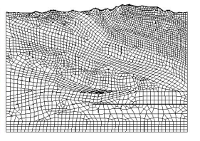
A partition of \(\Omega\) into hexahedrons: \(\mathcal{T} = \{ \Omega_k \}_{k=1}^{N}\), where the set of hexahedrons forms a conforming mesh of the domain (see Figure 1.1 for an example when \(d = 2\)),
-
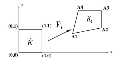
The unit cube \(K = [0, 1]^d\) and \(\hat{x} = (\hat{x}_i)_{i=1..d}\) the associated coordinate system,
-
\(F\), the vectorial application transforming \(K\) in \(\Omega_k\) (see Figure 1.2 for \(d = 2\)),
-
The space \(Q_r(K)\) of polynomials with real coefficients and variables in \(K\), where each variable is of degree less than or equal to \(r\), such that:
-
The approximation space
2.1. Spectral finite element method
By multiplying our equation by a test function \(\phi\) defined on \(\Omega\) and integrating by parts, we obtain the variational formulation:
Find \(p \in L^\infty(0, T; H^1_0(\Omega))\) such that:
We then approximate the solution \(p\) by a function \(p_h\) in the space \(U^d_r\) and we obtain the following discrete problem:
Find \(p_h \in L^\infty(0, T; U^d_r)\) such that:
The resulting mass matrix becomes densely populated as the simulation space expands and the order of approximation increases. This poses a double problem: a high computational load for the inversion of the matrix at each time step, and substantial data storage if we choose to retain the inverse of the mass matrix. These constraints underline the need for a more efficient method of handling large matrices in the context of acoustic simulation.
One solution to this problem is the use of Legendre-Gauss-Lobatto quadrature points for interpolation and the calculation of matrices by Gauss-Lobatto numerical integration, leading to mass condensation and enabling the use of an explicit scheme. This method is known as the "spectral finite element method". So the important point of this method is to make the interpolation points coincide with the quadrature points of the integration formulas.
3. The spectral mixed finite element method
We will reduce the storage of the stiffness matrix involved in the spectral finite element method by using a mixed form of equation.
3.1. Setting up a mixed formulation
We can write the equation in the following mixed forms:
-
\(\textit{System of first order equations}\):
Where \(F\) is the time primitive of the second member and \(v\) is the velocity of the fluid.
-
\(\textit{System of second order equations}\):
Where \(w\) is the acceleration of the fluid.
4. References
-
[1] Sandrine Fauqueux. Eléments finis mixtes spectraux et couches absorbantes parfaitement adaptées pour la propagation d’ondes élastiques en régime transitoire. Modélisation et simulation. ENSTA ParisTech, 2003. Français. NNT : 2003PA090002. tel-00007445
-
[2] Florent Pled, Christophe Desceliers. Review and Recent Developments on the Perfectly Matched Layer (PML) Method for the Numerical Modeling and Simulation of Elastic Wave Propagation in Unbounded Domains. Archives of Computational Methods in Engineering, 2022, 10.1007/s11831- 021-09581-y. hal-03196974