Solving linear elasticity using finite element method

1. Mathematical framework

In this section, we aim to solve the linear elasticity problem using the finite element method. We will first consider an isotropic medium and a homogeneous domain (which suits the test-case). This means determining the displacement field $u$ induced by the external force $f$ applied onto the deformable medium. The domain $\Omega \subset \mathbb{R}^3$, initially at rest, is the following:

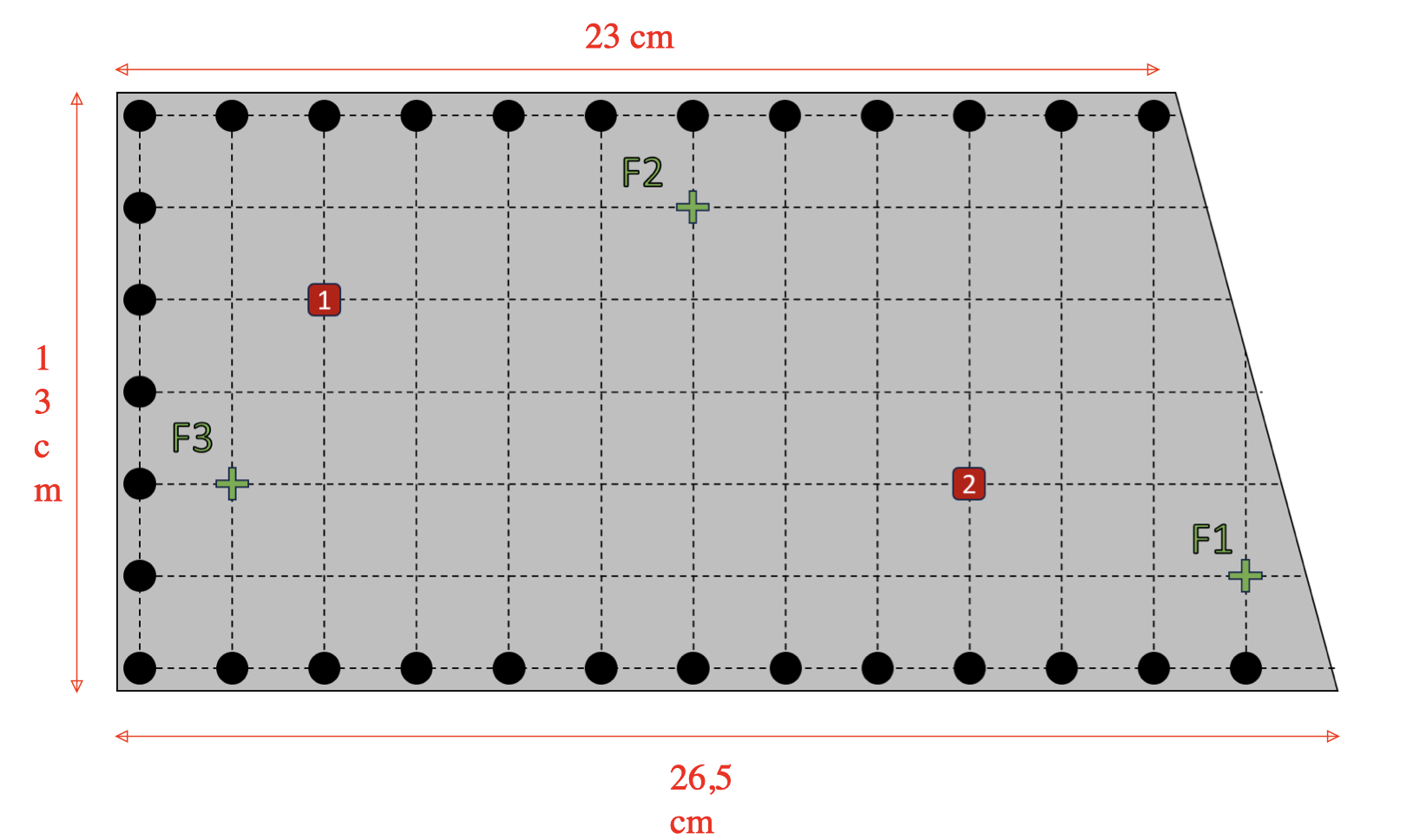
It is a rectangular steel plate with holes along the edges. The points F1, F2 and F3 are the ones where the force will be applied: a hammer will hit the plate at these points, which will be represented in our numerical model as a dirac source term (its intensity was determined thanks to a physical experiment).

First of all, we will consider the case of a homogeneous medium, which will further be extended to the case of an heterogeneous medium (nuclear vessel), where the material properties will vary in the domain.

Let us define the following quantities:

$\Omega \subset \mathbb{R}^3$ the domain of the problem
$\Gamma = \partial \Omega$ the boundary of the domain
$\sigma$ the stress field (constraints tensor)
$\varepsilon(u) = \frac{1}{2}(\nabla u + \nabla u^T)$ the linearized deformation field

In the case of static linear elasticity, we can define the equilibrium condition as:

\[\begin{equation} \nabla \cdot \sigma + f = 0 \quad \text{in } \Omega \end{equation}\]

where $f$ is the external force applied onto the deformable medium. In order to extend this condition to the dynamic case, we can use the Newton’s second law of motion:

\[\begin{equation} \rho \frac{\partial^2}{\partial t^2} u = \nabla \cdot \sigma + f \quad \text{in} \ \Omega \end{equation}\]

where $\rho$ is the mass density of the medium and $\frac{\partial^2}{\partial_{t^2}} u$ denotes the acceleration, in this case the second derivative with respect to time of the displacement field $u$, which will from now on be denoted by $u_{tt}$. This equation can be rewritten as:

\[\begin{equation} \rho u_{tt} - \nabla \cdot \sigma = f \quad \text{in} \ \Omega \end{equation}\]

In the case of linear elasticity, we can define the stress field as:

\[\begin{align*} \sigma &= \lambda \nabla \cdot u I + 2 \mu \varepsilon(u) \\ &= \lambda (\nabla \cdot u) I + \mu (\nabla u + \nabla u^T) \end{align*}\]

where $\lambda$ and $\mu$ are the Lamé coefficients, which are material properties of the medium. Since we are considering an homogeneous medium at first, we can safely assume that these coefficients are constant in the domain.

Finally, we can rewrite our problem in the case of dynamic linear elasticity as follows:

\[\begin{cases} \begin{align} \rho u_{tt} - \nabla \cdot \sigma &= f \quad \text{in} \ \Omega \\ \sigma &= \lambda (\nabla \cdot u) I + \mu (\nabla u + \nabla u^T) \\ \sigma \cdot n &= g \quad \text{on} \ \Gamma \\ u(x, 0) &= 0 \quad \text{in} \ \Omega \\ u_t(x, 0) &= 0 \quad \text{in} \ \Omega \end{align} \end{cases}\]

where $n$ is the outward unit normal vector to the boundary $\Gamma$.

1.1. Weak formulation

In order to solve this problem using the finite element method, we need to define the weak formulation of the first equation, which will then be handled by the finite element library FEEL++. Given the equation, we want to define a bilinear form $a(u, v)$ and a linear form $l(v)$ such that:

\[\begin{equation} a(u, v) = l(v) \quad \forall v \in V \end{equation}\]

where $V$ is a suitable function space. In order to do so, we can multiply the equation by a test function $v \in V$, integrate over the domain and apply the divergence theorem (in the case of a Riemannian manifold with boundary):

\[\begin{align} \int_{\Omega} \rho u_{tt} \cdot v \, dx - \int_{\Omega} \nabla \cdot \sigma \cdot v \, dx &= \int_{\Omega} f \cdot v \, dx \\ \int_{\Omega} \rho u_{tt} \cdot v \, dx + \int_{\Omega} \sigma : \nabla v \, dx - \int_{\Gamma} \sigma \cdot n \cdot v \, ds &= \int_{\Omega} f \cdot v \, dx \\ \int_{\Omega} \rho u_{tt} \cdot v \, dx + \int_{\Omega} \sigma : \varepsilon(v) \, dx &= \int_{\Omega} f \cdot v \, dx + \int_{\Gamma} g \cdot v \, ds \end{align}\]

where $\sigma : \varepsilon (v)$ denotes the maximal contraction of the tensors $\sigma$ and $\varepsilon(v)$, equal to $\sum_{i, j} \sigma_{ij} \varepsilon(v)_{ij}$. Proof:

Let us consider the 2D case (3D can be proven in the same manner). We start by defining:

\[\begin{align} u &= \begin{pmatrix} u_1 \\ u_2 \end{pmatrix} \\ \nabla \cdot u &= u_{1i} + u_{2j} \\ \end{align}\]

We denote by $u_{1i}$ the partial derivative of $u_1$ with respect to the $i$th variable. We can then rewrite the maximal contraction as:

\[\begin{align} \sigma(\mathbf{u}) : \nabla \mathbf{v} &= \left( (\lambda + 2 \mu)u_{1i} + \lambda u_{2j} \right)v_{1i} + \left( \mu (u_{1j} + u_{2i}) \right) v_{1j}\\ &+ \left( \mu (u_{1j} + u_{2i}) \right) v_{2i} + \left( \lambda u_{1i} + (\lambda + 2 \mu) u_{2j} \right) v_{2j}\\ \sigma(\mathbf{u}) : \varepsilon(\mathbf{v}) &= \left( (\lambda + 2 \mu ) u_{1i} + \lambda u_{2j} \right) v_{1i} + \left( \mu (u_{1j} + u_{2i}) \right) \cdot \frac{1}{2}(v_{1j} + v_{2i}) \\ &+ \left( \mu (u_{1j} + u_{2i}) \right) \cdot \frac{1}{2}(v_{1j} + v_{2i}) + \left( \lambda u_{1i} + (\lambda + 2 \mu) u_{2j} \right) v_{2j}\\ &= \left( (\lambda + 2 \mu)u_{1i} + \lambda u_{2j} \right)v_{1i} + \left( \mu (u_{1j} + u_{2i}) \right) v_{1j}\\ &+ \left( \mu (u_{1j} + u_{2i}) \right) v_{2i} + \left( \lambda u_{1i} + (\lambda + 2 \mu) u_{2j} \right) v_{2j}\\ \sigma(\mathbf{u}) : \nabla \mathbf{v} &= \sigma(\mathbf{u}) : \varepsilon(\mathbf{v}) \end{align}\]

In order to be able to solve for $u$, we need to define $a(u,v)$ and $l(v)$ as respectively a bilinear and a linear form. Therefore, we will rewrite the last equation as:

\[\begin{align} \sigma(\mathbf{u}) : \varepsilon(\mathbf{v}) &= \lambda(\nabla \mathbf{u})I : \varepsilon(\mathbf{v}) + 2\mu\varepsilon(\mathbf{u}) : \varepsilon(\mathbf{v}) \\ &= \lambda(\nabla \mathbf{u})(\nabla \mathbf{v}) + 2\mu\varepsilon(\mathbf{u}) : \varepsilon(\mathbf{v}) \end{align}\]

\[\begin{align} a(u, v) &= \int_{\Omega} \rho u_{tt} \cdot v \, dx + \int_{\Omega} \sigma : \varepsilon(v) \, dx \\ a(u, v) &= \int_{\Omega} \rho u_{tt} \cdot v \, dx + \int_{\Omega} \lambda(\nabla \mathbf{u})(\nabla \mathbf{v}) + 2\mu\varepsilon(\mathbf{u}) : \varepsilon(\mathbf{v}) \, dx \\ l(v) &= \int_{\Omega} f \cdot v \, dx + \int_{\Gamma} g \cdot v \, ds \end{align}\]

Which gives us the bilinear and linear forms we were looking for. We can now solve for $u$ using the finite element method.

But we wan’t to adapt it and approximate the second order derivative of the displacement field $u_{tt}$ by a second order centered finite difference scheme:

\[\begin{equation} u_{tt} \approx \frac{u_{n+1} - 2 u_n + u_{n-1}}{\Delta t^2} \end{equation}\]

where $u_n$ denotes the displacement field at the time $t = n \Delta t$.

1.1.1. Initial conditions

In order to compute the initial displacement fields $u^0$ and $u^1$, we can use the following second order Taylor expansion:

\[\begin{align} u_1 &= u_0 + \Delta t \partial_t u_0 + \frac{\Delta t^2}{2} \partial_t^2 u_0 + \mathcal{O}(\Delta t^3) \\ \int_\Omega u_1 \cdot v \, dx &= \int_\Omega u_0 \cdot v \, dx + \Delta t \int_\Omega \partial_t u_0 \cdot v \, dx + \frac{\Delta t^2}{2} \int_\Omega \partial_t^2 u_0 \cdot v \, dx + \mathcal{O}(\Delta t^3) \\ &= \frac{\Delta t^2}{2} \int_\Omega \partial_t^2 u_0 \cdot v \, dx + \mathcal{O}(\Delta t^3) \end{align}\]

Since the initial displacement field $u_0$ and the initial velocity field $\partial_t u_0$ are both equal to zero. Finally, we can solve for $u_1$ since we know that $u_0$ has to be the solution of:

\[\begin{equation} \partial_t^2 u_0 - \nabla \cdot \sigma = f_0 \quad \text{in} \ \Omega \end{equation}\]

Where $f_0$ represents the intial external force applied onto the medium (in our case defined by the dirac source term). We can then define the initial displacement field $u_0$ as the solution of the following problem:

\[\begin{align} \int_\Omega \partial_t^2 u^0 \cdot v \, dx - \int_\Omega \nabla \cdot \sigma(u_0) \cdot v \, dx &= \int_\Omega f_0 \cdot v \, dx \\ \int_\Omega \partial_t^2 u^0 \cdot v \, dx + \int_\Omega \sigma(u_0) : \nabla v \, dx - \int_\Gamma \sigma(u_0) \cdot n \cdot v \, ds &= \int_\Omega f_0 \cdot v \, dx \\ \int_\Omega \partial_t^2 u^0 \cdot v \, dx + \int_\Omega \sigma(u_0) : \varepsilon(v) \, dx &= \int_\Omega f_0 \cdot v \, dx + \int_\Gamma g_0 \cdot v \, ds \end{align}\]

Which gives us the following expression for $\partial_t^2 u^0$:

\[\begin{align} \int_\Omega \partial_t^2 u^0 \cdot v \, dx &= \int_\Omega f_0 \cdot v \, dx - \int_\Omega \sigma(u_0) : \varepsilon(v) \, dx + \int_\Gamma g_0 \cdot v \, ds \\ \int_\Omega \partial_t^2 u^0 \cdot v \, dx &= \int_\Omega f_0 \cdot v \, dx - \int_\Omega \lambda(\nabla u_0)(\nabla v) + 2\mu\varepsilon(u_0) : \varepsilon(v) \, dx + \int_\Gamma g_0 \cdot v \, ds \end{align}\]

We can then define the initial displacement field $u^1$ as the solution of the following problem:

\[\begin{align} \int_\Omega u_1 \cdot v \, dx &= \frac{\Delta t^2}{2 \rho} \int_\Omega \partial_t^2 u_0 \cdot v \, dx \\ &= \frac{\Delta t^2}{2 \rho} \left( \int_\Omega f_0 \cdot v \, dx - \int_\Omega \lambda(\nabla u_0)(\nabla v) + 2\mu\varepsilon(u_0) : \varepsilon(v) \, dx + \int_\Gamma g_0 \cdot v \, ds \right) \\ &= \frac{\Delta t^2}{2 \rho} \left( \int_\Omega f_0 \cdot v \, dx - \int_\Omega \lambda(\nabla u_0)(\nabla v) + 2\mu \mathbf{Tr} \left( \varepsilon(u_0) \varepsilon(v)^T \right) \, dx + \int_\Gamma g_0 \cdot v \, ds \right) \end{align}\]

1.1.2. Time discretization / loop

We can adapt the weak formulation to the time discretization scheme we want to use. In our case, we will use the centered finite difference scheme of order 2, which means that we will have to solve the following problem at each time step:

\[\begin{align} \int_\Omega \frac{u_{n+1} - 2 u_n + u_{n-1}}{\Delta t^2} \cdot v \, dx + \int_\Omega \sigma(u_n) : \varepsilon(v) \, dx - \int_\Gamma g \cdot v \, ds &= \int_\Omega f_n \cdot v \, dx \end{align}\]

But we want to solve for $u^{n+1}$, meaning we have to rewrite the equation as:

\[\begin{align} \int_\Omega u_{n+1} \cdot v \, dx &= \frac{\Delta t^2}{\rho} \left( \int_\Omega f \cdot v \, dx - \int_\Omega \sigma(u_n) : \varepsilon(v) \, dx + \int_\Gamma \sigma(u_n) \cdot n \cdot v \, ds \right) \\ &+ 2 \int_\Omega u_n \cdot v \, dx - \int_\Omega u_{n-1} \cdot v \, dx \\ \int_\Omega u_{n+1} \cdot v \, dx &= \frac{\Delta t^2}{\rho} \left( \int_\Omega f \cdot v \, dx - \int_\Omega \lambda(\nabla u_n)(\nabla v) + 2\mu\varepsilon(u_n) : \varepsilon(v) \, dx + \int_\Gamma g \cdot v \, ds \right) \\ &+ 2 \int_\Omega u_n \cdot v \, dx - \int_\Omega u_{n-1} \cdot v \, dx \end{align}\]

But we can simplify the equation by rewriting the maximal contraction. Let $\varepsilon(u_n)$ and $\varepsilon(v)$ be two $3 \times 3$ real matrices, with elements $\varepsilon(u_n)_{ij}$ and $epsilon(v)_{ij}$ respectively. The maximal contraction (double dot product) of $\sigma$ and $\varepsilon$ is defined as:

\[\begin{equation} \varepsilon(u_n) : \varepsilon(v) = \sum_{i=1}^{3} \sum_{j=1}^{3} \varepsilon(u_n)_{ij} \varepsilon(v)_{ij} \end{equation}\]

To express this using matrix operations, consider the trace of the product of $\varepsilon(u_n)$ and $\varepsilon(v)^T$ (the transpose of $\varepsilon(v)$):

\[\begin{equation} \text{Tr}(\varepsilon(u_n) \varepsilon(v)^T) = \sum_{i=1}^{3} (\varepsilon(u_n) \varepsilon(v)^T)_{ii} \end{equation}\]

The element $(\varepsilon(u_n) \varepsilon(v)^T)_{ii}$ is the dot product of the $i$th row of $\varepsilon(u_n)$ and the $i$th row of $\varepsilon(v)^T$. This is equivalent to the sum of the products of corresponding elements in the $i$th row of $\varepsilon(u_n)$ and the $i$th column of $\varepsilon(v)$:

\[\begin{equation} (\varepsilon(u_n) \varepsilon(v)^T)_{ii} = \sum_{j=1}^{3} \varepsilon(u_n)_{ij} \varepsilon(v)_{ji} \end{equation}\]

Therefore, the trace is:

\[\begin{equation} \text{Tr}(\varepsilon(u_n) \varepsilon(v)^T) = \sum_{i=1}^{3} \sum_{j=1}^{3} \varepsilon(u_n)_{ij} \varepsilon(v)_{ji} \end{equation}\]

Since $\varepsilon(v)^T$ has $\varepsilon(v)_{ji}$ as its $(i, j)$-element, the expression becomes:

\[\begin{equation} \text{Tr}(\varepsilon(u_n) \varepsilon(v)^T) = \sum_{i=1}^{3} \sum_{j=1}^{3} \varepsilon(u_n)_{ij} \varepsilon(v)_{ij} = \varepsilon(u_n) : \varepsilon(v) \end{equation}\]

Thus, we have shown that:

\[\begin{equation} \varepsilon(u_n) : \varepsilon(v) = \text{Tr}(\varepsilon(u_n) \varepsilon(v)^T) \end{equation}\]

Finally, we can rewrite the equation as:

\[\begin{align} \int_\Omega u_{n+1} \cdot v \, dx &= \frac{\Delta t^2}{\rho} \left( \int_\Omega f \cdot v \, dx - \int_\Omega \lambda(\nabla u_n)(\nabla v) + 2\mu \text{Tr} \left( \varepsilon(u_n) \varepsilon(v)^T \right) \, dx + \int_\Gamma g \cdot v \, ds \right) \\ &+ 2 \int_\Omega u_n \cdot v \, dx - \int_\Omega u_{n-1} \cdot v \, dx \end{align}\]

2. Using the Newmark beta method

In order to assure the stability of our scheme, the final implementation will use the Newmark beta model in order to perform the time integration. The method consists of solving the following two equations for $u_{n+1}$ and $\partial_t u_{n+1}$ respectively:

\[\begin{align} \begin{cases} u_{n+1} = u_n + \Delta t \partial_t u_n + \frac{\Delta t^2}{2} \left( (1 - 2 \beta) \partial_{tt} u_n + 2 \beta \partial_{tt} u_{n+1} \right) \\ \partial_t u_{n+1} = \partial_t u_n + \Delta t \left( (1 - \gamma) \partial_{tt} u_n + \gamma \partial_{tt} u_{n+1} \right) \end{cases} \end{align}\]

where $\beta$ and $\gamma$ are parameters of the method. Rearraging the terms, we can rewrite the equations as:

\[\begin{align} \partial_{tt} u_{n+1} = \frac{1}{\beta \Delta t^2} \left( u_{n+1} - u_n - \Delta t \partial_t u_n \right) - \frac{1 - 2 \beta}{2 \beta} \partial_{tt} u_n \\ \end{align}\]

But we already know that $u_{n+1}$ and $u_n$ are the respective solutions of the following problems:

\[\begin{align} \begin{cases} \rho \partial_{tt} u_{n+1} - \nabla \cdot \sigma(u_{n+1}) = f \\ \rho \partial_{tt} u_n - \nabla \cdot \sigma(u_n) = f \end{cases} \end{align}\]

The first can be expanded as:

\[\begin{align} \rho \int_\Omega \partial_{tt} u_{n+1} \cdot v \, dx + \int_\Omega \sigma(u_{n+1}) : \varepsilon(v) \, dx = \int_\Omega f \cdot v \, dx &+ \int_\Gamma g \cdot v \, ds \\ \rho \int_\Omega \frac{1}{\beta \Delta t^2} \left( u_{n+1} - u_n - \Delta t \partial_t u_n \right) \cdot v \, -\frac{1-2\beta}{2\beta} \partial_{tt} u_n \cdot v \, dx + \int_\Omega \sigma(u_{n+1}) : \varepsilon(v) \, dx &= \int_\Omega f \cdot v \, dx + \int_\Gamma g \cdot v \, ds \\ \rho \int_\Omega \frac{1}{\beta \Delta t^2} \left( u_{n+1} - u_n - \Delta t \partial_t u_n \right) \cdot v \, dx + \int_\Omega \sigma(u_{n+1}) : \varepsilon(v) \, dx = \int_\Omega f \cdot v \, dx &+ \int_\Gamma g \cdot v \, ds + \frac{1-2\beta}{2\beta} \int_\Omega \partial_{tt} u_n \cdot v \, dx \\ \int_\Omega \frac{\rho}{\beta \Delta t^2} u_{n+1} \cdot v \, dx + \int_\Omega \sigma(u_{n+1}) : \varepsilon(v) \, dx = \int_\Omega f \cdot v \, dx + \int_\Gamma g \cdot v \, ds &+ \frac{1-2\beta}{2\beta} \int_\Omega \partial_{tt} u_n \cdot v \, dx \\ + \frac{\rho}{\beta \Delta t^2} \int_\Omega u_n \cdot v \, dx &+ \frac{\rho}{\beta \Delta t} \int_\Omega \partial_t u_n \cdot v \, dx \end{align}\]

Knowing that $u_n$ is also solution to the dynamic linear elasticity problem, we have that:

\[\begin{align} \rho \int_\Omega \partial_{tt} u_n \cdot v \, dx + \int_\Omega \sigma(u_n) : \varepsilon(v) \, dx &= \int_\Omega f \cdot v \, dx + \int_\Gamma g \cdot v \, ds \\ \rho \int_\Omega \partial_{tt} u_n \cdot v \, dx &= \int_\Omega f \cdot v \, dx + \int_\Gamma g \cdot v \, ds - \int_\Omega \sigma(u_n) : \varepsilon(v) \, dx \\ \rho \int_\Omega \partial_{tt} u_n \cdot v \, dx &= \int_\Omega f \cdot v \, dx - \int_\Omega \lambda(\nabla u_n)(\nabla v) + 2\mu\varepsilon(u_n) : \varepsilon(v) \, dx + \int_\Gamma g \cdot v \, ds \\ \int_\Omega \partial_{tt} u_n \cdot v \, dx &= \frac{1}{\rho} \int_\Omega f \cdot v \, dx - \frac{1}{\rho} \int_\Omega \lambda(\nabla u_n)(\nabla v) + 2\mu \text{Tr} \left( \varepsilon(u_n) \varepsilon(v)^T \right) \, dx + \frac{1}{\rho} \int_\Gamma g \cdot v \, ds \end{align}\]

Which leads us to the equation:

\[\begin{align} \int_\Omega \frac{\rho}{\beta \Delta t^2} u_{n+1} \cdot v \, dx &+ \int_\Omega \sigma(u_{n+1}) : \varepsilon(v) \, dx = \int_\Omega f \cdot v \, dx + \int_\Gamma g \cdot v \, ds + \frac{\rho}{\beta \Delta t^2} \int_\Omega (u_n + \Delta t \partial_t u_n) \cdot v \, dx \\ &+ \rho \frac{1-2\beta}{2\beta} \int_\Omega \partial_{tt} u_n \cdot v \, dx \\ &= \int_\Omega f \cdot v \, dx + \int_\Gamma g \cdot v \, ds + \frac{\rho}{\beta \Delta t^2} \int_\Omega (u_n + \Delta t \partial_t u_n) \cdot v \, dx \\ &+ \frac{1-2\beta}{2\beta} \left( \int_\Omega f \cdot v \, dx - \int_\Omega \lambda(\nabla u_n)(\nabla v) + 2\mu \text{Tr} \left( \varepsilon(u_n) \varepsilon(v)^T \right) \, dx + \int_\Gamma g \cdot v \, ds \right) \end{align}\]

Finally we have the form:

\[\begin{align} \int_\Omega \frac{\rho}{\beta \Delta t^2} u_{n+1} \cdot v \, dx &+ \int_\Omega \lambda(\nabla u_{n+1})(\nabla v) + 2\mu \text{Tr} \left( \varepsilon(u_{n+1}) \varepsilon(v)^T \right) \, dx \\ & = \int_\Omega f \cdot v \, dx + \int_\Gamma g \cdot v \, ds + \frac{\rho}{\beta \Delta t^2} \int_\Omega (u_n + \Delta t \partial_t u_n) \cdot v \, dx \\ &+ \rho \frac{1-2\beta}{2\beta} \left( \int_\Omega f \cdot v \, dx - \int_\Omega \lambda(\nabla u_n)(\nabla v) + 2\mu \text{Tr} \left( \varepsilon(u_n) \varepsilon(v)^T \right) \, dx + \int_\Gamma g \cdot v \, ds \right) \end{align}\]

2.1. Computing the initial displacement fields

The last equation can be used in order to compute $u_1$ since the initial displacement field $u_0$ and its velocity are known as equal to zero. We can then define the initial displacement field $u_1$ as the solution of the following problem:

\[\begin{align} \frac{\rho}{\beta \Delta t^2} \int_\Omega u_1 \cdot v \, dx &+ \int_\Omega \lambda(\nabla u_1)(\nabla v) + 2\mu \text{Tr} \left( \varepsilon(u_1) \varepsilon(v)^T \right) \, dx = \int_\Omega f_0 \cdot v \, dx + \int_\Gamma g \cdot v \, ds \\ &+ \frac{1 - 2\beta}{2\beta} \int_\Omega f \cdot v \, dx + \frac{1 - 2\beta}{2\beta} \int_\Gamma g \cdot v \, ds \\ &- \frac{1 - 2\beta}{2\beta} \int_\Omega \lambda(\nabla u_0)(\nabla v) + 2\mu \text{Tr} \left( \varepsilon(u_0) \varepsilon(v)^T \right) \, dx \end{align}\]

But in order to start iterating over the time steps, we also need to compute and store the velocities of our displacement fields, starting by computing $\partial_t u_1$ thanks to the equation from the Newmark beta method:

\[\begin{align} \partial_t u_1 &= \partial_t u_0 + \Delta t \left( (1 - \gamma) \partial_{tt} u_0 + \gamma \partial_{tt} u_1 \right) \\ \partial_t u_1 &= \Delta t \left( (1 - \gamma) \partial_{tt} u_0 + \gamma \partial_{tt} u_1 \right) \\ \end{align}\]

But we have that:

\[\begin{align} \begin{cases} \int_\Omega \partial_{tt} u_0 \cdot v &= \frac{1}{\rho} \int_\Omega f_0 \cdot v \, dx - \frac{1}{\rho} \int_\Omega \lambda(\nabla u_0)(\nabla v) + 2\mu \text{Tr} \left( \varepsilon(u_0) \varepsilon(v)^T \right) \, dx + \frac{1}{\rho} \int_\Gamma g \cdot v \, ds \\ \int_\Omega \partial_{tt} u_1 \cdot v &= \frac{1}{\rho} \int_\Omega f_1 \cdot v \, dx - \frac{1}{\rho} \int_\Omega \lambda(\nabla u_1)(\nabla v) + 2\mu \text{Tr} \left( \varepsilon(u_1) \varepsilon(v)^T \right) \, dx + \frac{1}{\rho} \int_\Gamma g \cdot v \, ds \end{cases} \end{align}\]

And we already computed $u_1$ before, so the following equation can be solved thanks to feel++:

\[\begin{align} \int_\Omega \partial_t u_1 \cdot v &= \Delta t \left( (1 - \gamma) \int_\Omega \partial_{tt} u_0 \cdot v \, dx + \gamma \int_\Omega \partial_{tt} u_1 \cdot v \, dx \right) \\ \int_\Omega \partial_t u_1 \cdot v &= \Delta t \left(\frac{1 - \gamma }{\rho} \left( \int_\Omega f_0 \cdot v \, dx - \int_\Omega \lambda(\nabla u_0)(\nabla v) + 2\mu \text{Tr} \left( \varepsilon(u_0) \varepsilon(v)^T \right) \, dx + \int_\Gamma g \cdot v \, ds \right) \right. \\ &+ \left.\frac{\gamma}{\rho} \left( \int_\Omega f_1 \cdot v \, dx - \int_\Omega \lambda(\nabla u_1)(\nabla v) + 2\mu \text{Tr} \left( \varepsilon(u_1) \varepsilon(v)^T \right) \, dx + \int_\Gamma g \cdot v \, ds \right) \right) \\ \end{align}\]

2.2. Time discretization / loop

During the time loop, we will also have to compute the velocity $\partial_t u_{n+1}$ at each time step in order to be able to use it during the following one. As before, we will first solve for $u_{n+1}$ with $partial_t u_n$, and use it in order to compute $\partial_t u_{n+1}$:

\[\begin{align} \int_\Omega \partial_t u_{n+1} \cdot v \, dx &= \Delta t \left( (1 - \gamma) \int_\Omega \partial_{tt} u_n \cdot v \, dx + \gamma \int_\Omega \partial_{tt} u_{n+1} \cdot v \, dx \right) \\ \int_\Omega \partial_t u_{n+1} \cdot v \, dx &= \Delta t \left(\frac{1 - \gamma}{\rho} \left( \int_\Omega f_n \cdot v \, dx - \int_\Omega \lambda(\nabla u_n)(\nabla v) + 2\mu \text{Tr} \left( \varepsilon(u_n) \varepsilon(v)^T \right) \, dx + \int_\Gamma g \cdot v \, ds \right) \right. \\ &+ \left. \frac{\gamma}{\rho} \left( \int_\Omega f_{n+1} \cdot v \, dx - \int_\Omega \lambda(\nabla u_{n+1})(\nabla v) + 2\mu \text{Tr} \left( \varepsilon(u_{n+1}) \varepsilon(v)^T \right) \, dx + \int_\Gamma g \cdot v \, ds \right) \right) \\ \end{align}\]

This value is computed thanks to feel++ and stored in the variable $dtu_n$. It will be used in order to compute $u_{n+2}$, here denoted $u_{n+1}$, at the following iteration:

\[\begin{align} \int_\Omega \frac{\rho}{\beta \Delta t^2} u_{n+1} \cdot v \, dx &+ \int_\Omega \lambda(\nabla u_{n+1})(\nabla v) + 2\mu \text{Tr} \left( \varepsilon(u_{n+1}) \varepsilon(v)^T \right) \, dx \\ & = \int_\Omega f \cdot v \, dx + \int_\Gamma g \cdot v \, ds + \frac{\rho}{\beta \Delta t^2} \int_\Omega (u_n + \Delta t \partial_t u_n) \cdot v \, dx \\ &+ \frac{1-2\beta}{2\beta} \left( \int_\Omega f \cdot v \, dx - \int_\Omega \lambda(\nabla u_n)(\nabla v) + 2\mu \text{Tr} \left( \varepsilon(u_n) \varepsilon(v)^T \right) \, dx + \int_\Gamma g \cdot v \, ds \right) \end{align}\]

2.3. Boundary conditions

In order to verify the correctness of our implementation, we will also have to apply the boundary conditions to our problem with respect to the physical experiment conducted by sonorhc. Therefore, we will have to apply the following boundary conditions to our problem:

\[\begin{align} \begin{cases} u = 0 & \text{on} \ \Gamma \\ \sigma \cdot n = 0 & \text{on} \ \Gamma \end{cases} \end{align}\]

Since our metal plate is attached to a rigid support, we can assume that the displacement field $u$ is equal to zero on the boundary $\Gamma$. We set $\sigma \cdot n = 0$ in order to ensure that no external stress is applied to the boundary of the plate.

2.4. Implementation of Newmark model using Feel++

Now that the mathematical framework has been defined, we can implement the problem using the finite element library Feel++. This will only be focused on the numerical implementation, the results can be obtained as explained in the next section. We will start by implementing the Newmark beta model in order to compute our initial displacement field $u_1$ and its velocity $\partial_t u_1$:

////////////////////////////////////////////////////
//          Newmark beta-model for dtun           //
////////////////////////////////////////////////////
l_.zero();
a_.zero();

a_ += integrate( _range = elements(mesh_), _expr= rho / time_step / time_step / beta * trans(idt(u_))*id(v_)
                                            + lambda * inner(grad(u_), grad(v_)) + 2 * mu * trace(sym(grad(u_)*trans(sym(grad(v_))))));
l_ += f_0;
l_ += integrate( _range = elements(mesh_), _expr= rho * (1 - 2*beta)/(2*beta) * inner(f,id(v_)) );
l_ += integrate( _range = elements(mesh_), _expr= - rho * (1 - 2*beta)/(2*beta) * lambda * inner(gradv(u0_),grad(v_))
                                            - rho * (1 - 2*beta)/(beta) * mu * trace(sym(gradv(u0_)) * trans(sym(grad(v_)))));
l_ += integrate( _range = markedfaces(mesh_, "Gamma"), _expr= (1 + rho * (1-2*beta)/(2*beta) * inner(g, id(v_)))); // = (1 + (1 - 2*beta)/(2*beta) * inner(g, id(v_)));

a_.solve( _rhs = l_, _solution = u_ );

////////////////////////////////////////////////////
//         Newmark gamma-model for dtun           //
////////////////////////////////////////////////////
a_.zero();
l_.zero();

a_ += integrate( _range = elements(mesh_), _expr= trans(idt(dtun))*id(v_) );
l_ += f_0; // f_0.scale(time_step*(1-gamma)/rho);
l_ += integrate( _range = elements(mesh_), _expr= time_step * (1-gamma) / rho *(-lambda*inner(gradv(u0_),grad(v_)) - 2*mu*trace(sym(gradv(u0_))*trans(sym(grad(v_)))) )  );
l_ += integrate( _range = elements(mesh_), _expr= time_step * gamma / rho * (inner(f,id(v_)) - lambda*inner(gradv(u_),grad(v_)) - 2*mu*trace(sym(gradv(u_))*trans(sym(grad(v_))))));
l_ += integrate( _range = markedfaces(mesh_, "Gamma"), _expr= 1/rho * inner(g, id(v_)) );

a_.solve( _rhs = l_, _solution = dtun );

In the same manner, we will compute the displacement field $u_{n+1}$ at each time step using the following code:

// u_ = u_n+1
// dtun holds the last velocity of the displacement field u
auto un = bdf_->unknown(0); // un = u_n
auto un_1 = bdf_->unknown(1);  // un_1 = u_{n-1}

auto dt = expr(bdf_->timeStep());

////////////////////////////////////////////////////
//          Newmark beta-model for dttun          //
////////////////////////////////////////////////////
at_ += integrate( _range = elements(mesh_), _expr= rho / dt / dt / beta * trans(idt(u_))*id(v_)
                                            + lambda * inner(grad(u_), grad(v_)) + 2 * mu * trace(sym(gradv(u_))*trans(sym(grad(v_)))));
lt_ += integrate( _range = elements(mesh_), _expr= inner(f,id(v_)) + rho / beta / dt / dt * inner(id(un) + dt * id(dtun), id(v_)));
lt_ += integrate( _range = elements(mesh_), _expr= (1 - 2*beta)/(2*beta) * inner(f,id(v_))
                                            - (1 - 2*beta)/(2*beta) * lambda * inner(gradv(un),grad(v_))
                                            - (1 - 2*beta)/(beta) * mu * trace(sym(grad(un)*trans(sym(grad(v_))))));
lt_ += integrate( _range = markedfaces(mesh_, "Gamma"), _expr= 1/(2*beta) *inner(g, id(v_))); // = (1 + (1 - 2*beta)/(2*beta) * inner(g, id(v_)));
at_.solve( _rhs = lt_, _solution = u_ );
this->exportResults();

////////////////////////////////////////////////////
//         Newmark gamma-model for dtun           //
////////////////////////////////////////////////////
at_.zero();
lt_.zero();

at_ += integrate( _range = elements(mesh_), _expr = trans(idt(dtun)) * id(v_) );
lt_ += integrate( _range = elements(mesh_), _expr = dt * (1-gamma) / rho * inner(f,id(v_)) );
lt_ += integrate( _range = elements(mesh_), _expr = - dt * (1-gamma) / rho * (lambda * inner(gradv(un),grad(v_)) - 2*mu*trace(sym(gradv(un))*trans(sym(grad(v_))))));
lt_ += integrate( _range = elements(mesh_), _expr = dt * gamma / rho * (inner(f,id(v_)) - (lambda * inner(gradv(u_),grad(v_)) - 2*mu*trace(sym(gradv(u_))*trans(sym(grad(v_)))))));
lt_ += integrate( _range = markedfaces(mesh_, "Gamma"), _expr = 1/rho * inner(g, id(v_)) );

at_.solve( _rhs = lt_, _solution = dtun );

The values of $u_{n}$ and $\partial_t u_{n}$ are stored in the variables $un$ and $dtun$ respectively, and will be used in order to compute $u_{n+1}$ and $\partial_t u_{n+1}$ at the following iteration. They are automatically updated at each iteration thanks to the bdf structure, serving as result holder.

Finally, we will apply the boundary conditions to our problem using the following code:

template <int Dim, int Order>
void Elastic<Dim, Order>::processBoundaryConditions()
{
    // Boundary Condition Dirichlet
    auto bc_dir = specs_["/BoundaryConditions/elastic/Dirichlet/Gamma/g/expr"_json_pointer].get<std::string>();
    std::cout << "BoundaryCondition Dirichlet : " << bc_dir << std::endl;
    a_+=on(_range=markedfaces(mesh_,"Gamma"), _rhs=l_, _element=u_, _expr=expr<FEELPP_DIM,1>( bc_dir ) );

    // Boundary Condition Neumann
    auto bc_neu = specs_["/BoundaryConditions/elastic/Neumann/Gamma/pure_traction/g/expr"_json_pointer].get<std::string>();
    std::cout << "Boundary Condition Neumann : " <<  bc_neu << std::endl;
    l_ += integrate( _range = markedfaces( mesh_ , "Gamma"), _expr = inner( expr<FEELPP_DIM,1>( bc_neu ), id( v_ )) );
}

3. Implementation using Feel++

Now that the mathematical framework has been defined, we can implement the problem using the finite element library Feel++. First, we will initialize our environment using vectorial spaces:

using mesh_t = Mesh<Simplex<Dim>>;
using space_t = Pchv_type<mesh_t, Order>;
using space_ptr_t = Pchv_ptrtype<mesh_t, Order>;
using element_ = typename space_t::element_type;
using form2_type = form2_t<space_t,space_t>;
using form1_type = form1_t<space_t>;
using bdf_ptrtype = std::shared_ptr<Bdf<space_t>>;
using exporter_ptrtype = std::shared_ptr<Exporter<mesh_t>>;

3.1. Initial conditions

Then, we will start be computing our initial displacement fields $u_0$ and $u_1$ using the following code:

E = get_value(specs_, "/Parameters/elastic/E/expr", 1.0e9); // Young modulus
nu = get_value(specs_, "/Parameters/elastic/nu/expr", 0.3); // Poisson ratio
rho = get_value(specs_, "/Parameters/elastic/rho/expr", 7800.0); // Density in kg.m^-3 (default : steel)
lambda = E*nu/( (1+nu)*(1-2*nu) );
mu = E/(2*(1+nu));
F = specs_["/InitialConditions/elastic/externalF/Expression/Omega/expr"_json_pointer].get<std::string>();
G = specs_["/BoundaryConditions/elastic/Gamma/g/expr"_json_pointer].get<std::string>();
std::string DTU0 = specs_["/InitialConditions/elastic/displacement/Expression/Omega/expr"_json_pointer].get<std::string>();
auto f = expr<FEELPP_DIM,1>(F);
auto g = expr<FEELPP_DIM,1>(G);
auto dtu0 = expr<FEELPP_DIM,1>(DTU0);
auto u0_ = Xh_->element();

node_type n(FEELPP_DIM);
for (int i = 0 ; i < FEELPP_DIM ; i++){
    n(i) = 0.1;
}
auto s = std::make_shared<SensorPointwise<space_t>>(Xh_, n, "S");
auto f_0 = form1( _test = Xh_, _vector = s->containerPtr() );

double rho = 7800.; // kg.m^-3

l_.zero();
a_.zero();
a_ += integrate( _range = elements(mesh_), _expr=trans(idt(u_))*id(v_)); //1
f_0 += integrate(_range = elements(mesh_), _expr = -time_step * time_step / rho / 2 * lambda * inner(gradv(u0_),grad(v_))); //3
f_0 += integrate(_range = elements(mesh_), _expr = -time_step * time_step / rho * mu * trace(sym(gradv(u0_)) * trans(sym(grad(v_))))); //4
f_0 += integrate(_range = markedfaces(mesh_, "Gamma"), _expr = time_step * time_step / rho / 2 * inner(g, id(v_))); //5
a_.solve( _rhs = f_0, _solution = u_ );

bdf_ = Feel::bdf( _space = Xh_, _steady=steady, _initial_time=initial_time, _final_time=final_time, _time_step=time_step, _order=time_order );
bdf_->start();
if ( steady )
    bdf_->setSteady();
bdf_->initialize( u0_ ); // set u0_
bdf_->shiftRight( u_ ); // set u1_

The contribution of the dirac is directly embeded in the linear form $f_0$ and will be used in order to compute $u_1$.

3.2. Time discretization / loop

We will compute the displacement field $u_{n+1}$ at each time step using the following code:

auto un = bdf_->unknown(0); // un = u_n
auto un_1 = bdf_->unknown(1);  // un_1 = u_{n-1}

auto dt = expr(bdf_->timeStep());

at_ += integrate( _range = elements(mesh_), _expr = trans(idt(u_))*id(v_) );

lt_ += integrate( _range = elements(mesh_), _expr = dt*dt/rho * inner(f,id(v_))); //1
lt_ += integrate( _range = elements(mesh_), _expr = -dt*dt/rho * lambda * inner(gradv(un),grad(v_))); //2
lt_ += integrate( _range = elements(mesh_), _expr = -dt*dt/rho * 2 * mu * trace(sym(gradv(un)) * trans(sym(grad(v_)) ))); //3
lt_ += integrate( _range = markedfaces(mesh_, "Gamma"), _expr = dt*dt/rho * inner(g, id(v_))); //4
lt_ += integrate( _range = elements(mesh_), _expr = 2*inner(id(un),id(v_)) - inner(id(un_1),id(v_))); //5

at_.solve( _rhs = lt_, _solution = u_ );

this->exportResults();

at_.zero();
lt_.zero();

3.3. Execution

One can execute the code using the following command:

cd build/default/src &&
./feelpp_fs_elasticity --config-file ../../../src/cases/elastic/elastic.cfg

The results are automatically exported to the feelpp database, it’s location is given at the end of the execution in the terminal.

3.4. Results

The results are stored as an ensight format, which can be visualized using Paraview. Since the results are displacement fields, we can either visualize them using the 'Glyph' or the 'Warp by vector' filter (which can retrieved in the menu unde 'Filter' > 'Alphabetical' > 'Glyph' or 'Warp by vector').

3.5. Testcase

The first test was done on the same square.geo file that was used for the acoustic wave equation, a 2D representation of a square of size 2.

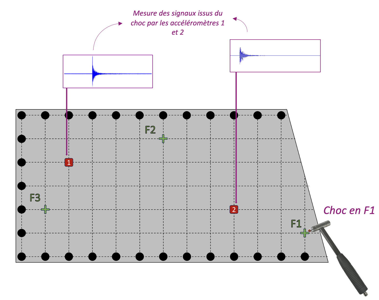
The second one was to study the correctness of the code by comparing the numerical results with measurements taken during a physical experiment. The experiment consisted in hitting a steel plate (mass density rho of 7800 kg/m^3) with a hammer at three different points (F1, F2 and F3), and measuring the time it took for the disturbance / wave to reach points 1 and 2. The Young’s modulus and the Poisson’s ratio associated to the problem were given to us, and are respectively equal to 210 Gpa = 2.1e11 pa and 0.3. Here is the setup of the experiment:

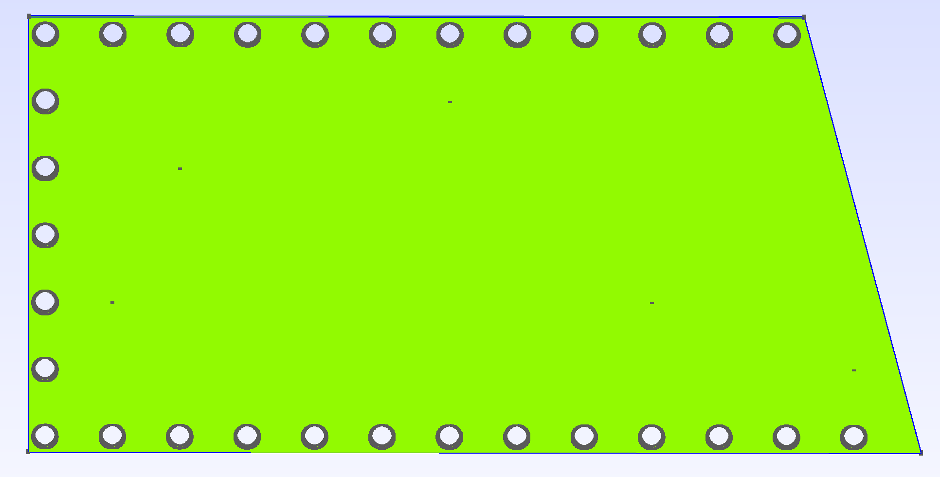
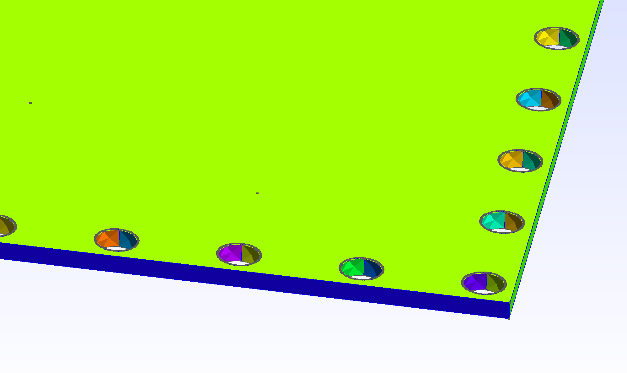
The template was given in a .step format, which had to be converted to a .geo file to adapt to feelpp’s restrictions. The final model is the following:

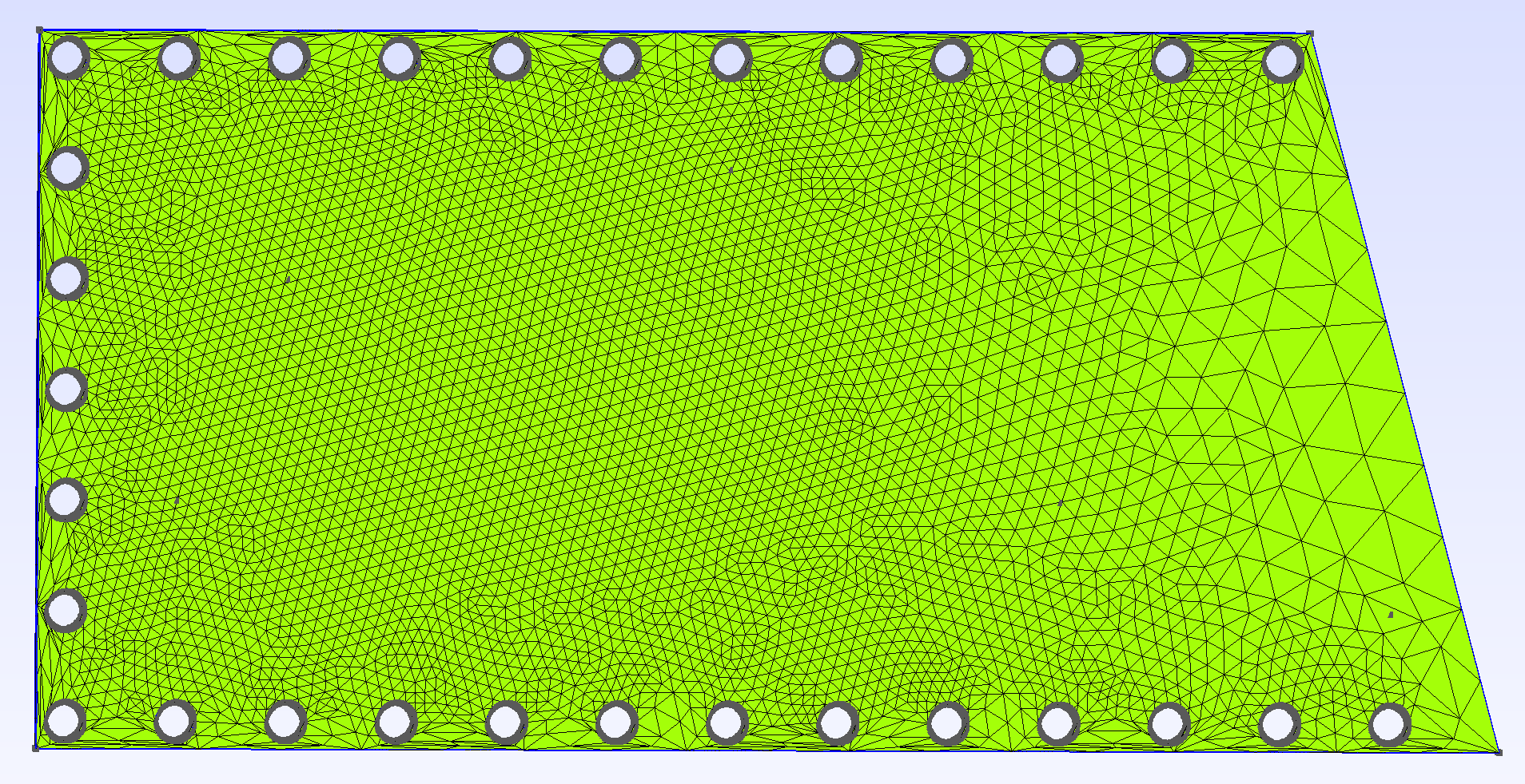
The boundary had to consider the holes in the plate, which were modeled as cylinders, and could therefore be properly meshed if given the right mesh size (in our configuration file 0.02 was used in order to present suitable results along the complex boundary); this can of course be modified to have the desired accuracy using the json configuration file. The final mesh is the following:

The boundary of the domain (Gamma) was also created alongside of two groups, Dirac and PointsOfInterests, respectively corresponding to the points where the force is applied and the points where the measurements are taken. Their repartition is visible on the following image: