Wave equation using CFPDEs Toolbox

1. Problem Statement

The unique thing about $\texttt{CFPDEs}$ is that it allows you to specify the PDE problem to be solved using a configuration file format: $\texttt{JSON}$ . These configuration files define the mathematical models, boundary and initial conditions, parameters, domain, and other necessary information to describe the problem. This makes $\texttt{CFPDEs}$ very flexible and adaptable to a wide range problems.

Our project focuses on simulating acoustic wave propagation in a 2D urban environment. Our approach involves transforming the classic second-order acoustic wave equation into a first-order system to be compatible with the $\texttt{CFPDEs toolbox}$, which primarily handles first-order partial differential equations $\texttt{(PDEs).}$

The general form of the equation is given by:

\[ d\partial_t u + \nabla.(-c\nabla u -\alpha u +\gamma) + \beta \nabla u + u = f\]

where:

$u$ : is the unknown quantity that we are trying to solve for.
$d$ : is the diffusion coefficient.
$c$ : is the convection coefficient.
$\alpha$ : is the damping coefficient..
$\beta$ : is the stress coefficient.
$\gamma$ : is the source coefficient.
$a$ : is the reaction coefficient.
$f$ : is the forcing term.

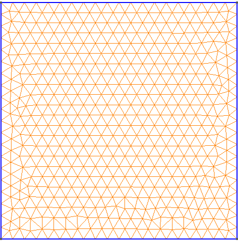
The urban environment is represented in our first test by a simple square and other geometry in a 2D plane.

Figure 1. Geometry of 2D square

The classic acoustic wave equation is given by:

\[\frac{\partial^2 p}{\partial t^2} - c^2 \nabla^2 p = 0\]

where $p$ is the acoustic pressure and $c$ is the speed of sound.

To adapt this to a first-order system, we introduce the velocity $v = \frac{\partial p}{\partial t}$. Thus, the equation is transformed into:

\[\begin{cases} \frac{\partial p}{\partial t} - v = 0 \\ \frac{\partial v}{\partial t} - c^2 \nabla^2 p = 0 \end{cases} \implies \begin{cases} \frac{\partial p}{\partial t} - v = 0 \\ \frac{\partial v}{\partial t} + \nabla \cdot (-c^2 \nabla p) = 0 \end{cases}\]

This formulation is compatible with the $\texttt{CFPDEs toolbox}$, which requires first-order $\texttt{PDEs}$.

Comparing the wave equation with the general form of the equation, we get the following identification:

For the first equation:

$u = p$ : is the acoustic pressure.
$d = 1$ : is the diffusion coefficient.
$c = a = \alpha = \beta = \gamma = 0$
$f = v$ : is the forcing term.

For the second equation:

$u = v$ : is the velocity.
$d = 1$ : is the diffusion coefficient.
$\gamma = -c^2 \nabla p$ : is the source coefficient.
$\alpha = \beta = c = a = f = 0$

2. Implémentation

The $\texttt{JSON}$ file configures the following:

JSON Configuration

Models(cfpdes) : Definition of the equations (equation1 for pressure, equation2 for velocity).
Parameters (Parameters): Sound speed (c) and parameters for initial conditions.
Mesh (Meshes): Specifications for importing and sizing the mesh.
Initial and Boundary Conditions (InitialConditions, BoundaryConditions): Definitions of initial values for pressure and velocity, and boundary conditions.

JSON Configuration for the square

{
    "Name": "Onde",
    "ShortName": "onde",
    "Models":
    {
        "cfpdes":{
            "equations":["equation1","equation2"]
        },
        "equation1":{
            "setup":{
                "unknown":{
                    "basis":"Pch1",
                    "name":"pressure",
                    "symbol":"p"
                },
                "coefficients":{
                    "d": "1",
                    "f":"equation2_v:equation2_v"
                }
            }
        },
        "equation2":{
            "setup":{
                "unknown":{
                    "basis":"Pch1",
                    "name":"velocity",
                    "symbol":"v"
                },
                "coefficients":{
                    "d": "1.0",
                    "gamma": "{-c^2*equation1_grad_p_0, -c^2*equation1_grad_p_1}:c:equation1_grad_p_0:equation1_grad_p_1"
                }
            }
        }
    },
    "Parameters": {
        "c": 4,
        "x0":1,
        "y0":1,
        "sigma":0.05,
        "a": 0.3
    },
    "Meshes":
    {
        "cfpdes":
        {
            "Import":
            {
                "filename":"$cfgdir/geo/square2d.geo",
                "hsize":0.01
            }
        }
    },
    "Materials":
    {
        "mymat":
        {
            "markers":"Omega"
        }
    },
    "BoundaryConditions":{
        "equation1": {
          "Neumann": {
            "mybc": {
              "markers": ["Left", "Right","Bottom","Top"],
              "expr": "0"
            }
          }
        },
        "equation2": {
          "Neumann": {
            "mybc": {
              "markers": ["Left", "Right","Bottom","Top"],
              "expr": "0"
            }
          }
        }
    },
    "InitialConditions":{
        "equation1":{
            "pressure": {
                "Expression": {
                    "myic": {
                        "markers": "Omega",
                        "expr": "a * exp(-((x-x0)^2 + (y-y0)^2)/(2*sigma^2)):a:x0:y0:sigma:x:y"
                    }
                }
            }
        },
        "equation2":{
            "velocity":{
                "Expression": {
                    "myic": {
                        "markers": "Omega",
                        "expr": "0"
                    }
                }
            }
        }
    },
    "PostProcess":
    {
        "cfpdes":
        {
            "Exports":
            {
                "fields":["all"]
            }
        }
    }
}

The CFG file is used to configure the execution:

CFG Configuration

Directory and Dimension: Settings for the working directory and the dimension of the simulation.
JSON File Path: Specification of the $\texttt{JSON}$ file to use.
Solver Configuration: Choice of solver and parameters for monitoring the solution.

CFG Configuration for the square

directory=onde
case.dimension=2

[cfpdes]
filename=$cfgdir/onde.json

verbose=1

solver=Newton#Picard
ksp-monitor=0
snes-monitor=1

[cfpdes.equation1]
time-stepping=Theta

[cfpdes.equation2]
time-stepping=Theta

[ts]
time-initial=0
time-step=0.003
time-final=1
restart.at-last-save=true

3. Simulation Process

The simulation can be executed using either Docker or on a computing cluster. The following outlines the steps for each method:

3.1. Using Docker

Docker offers a convenient and isolated environment for running the simulation. Follow these steps to execute the simulation using Docker:

Pulling the Docker Image: Begin by pulling the Feel++ Docker image using the command:

docker run --rm -it -v $HOME/feel:/feel ghcr.io/feelpp/feelpp:jammy

This command downloads the Feel++ image and mounts your $HOME/feel directory to the Docker container for persistent data storage.

Running the Simulation: Inside the Docker container, launch the simulation with:

feelpp_toolbox_coefficientformpdes --config-file onde.cfg

This command initiates the simulation using the settings defined in onde.cfg.

Retrieving Simulation Results: After the simulation is complete, retrieve the results from the Docker container:

cp -R ~/feelppdb/onde /feel/

This step copies the simulation results to the mounted directory, making them accessible outside the Docker container.

Visualizing Results in ParaView: Open the results in ParaView for visualization and analysis.

3.2. On a Computing Cluster

For those with access to a computing cluster with Feel++ installed, the simulation can be executed directly on the cluster:

Accessing the Cluster: Log into your cluster where Feel++ is already installed.
Executing the Simulation: Run the simulation using the same command as you would in Docker:

feelpp_toolbox_coefficientformpdes --config-file onde.cfg

Ensure that onde.cfg and square2d.geo are accessible on the cluster.

3.3. Post-Processing

Regardless of the execution method (Docker or cluster), after the simulation is completed, the results need to be collected and analyzed. If using Cluster, remember to transfer the output data from the Cluster container to your host machine for further processing.