IBAT

Table of Contents

1. Available Data
2. Data Selection
3. Modelling & Simulations
- 3.1. Exercise Intensity
- 3.2. Choice of Simulation Cases
References

1. Available Data

A total of 200 sensor nodes have been placed inside the university building, where over 75 sensor nodes are dedicated to the building energy application. They measure temperature, relative humidity, noise, presence and light intensity at a frequency of 1 measure per second. Recently, 4fastsim sensors, which collect temperature data, were installed in the 3 rooms we will consider for our modelling. All these collected data are stored in an Elasticsearch database. [IB]

Figure 1. Sensors Location (Source: Zohra Djatouti & Guillaume Schreiner)

2. Data Selection

In order to find out which input value to use for the different parameters contained in the Pulse environment file, we will make use of the data available to us and of additional documentation.

Air Velocity:
We will use as reference value \(0.1\; m/s\) as this value may be used as the assumed internal air velocity in some simple heat transfer calculations. [AV]

Ambient Temperature:
We will use the temperature data from our data sets.

Atmospheric Pressure:
In order to calculate the atmospheric pressure, we need to know the altitude. Thus, using Google Earth, we find \(140\; m\) as the altitude at the bottom of the building and \(157\; m\) at the top of the building. We will therefore set \(149\; m\) as the approximate altitude of the 3 rooms.

Clothing Resistance:
Concerning clothing resistance we have no data available in our data sets. By searching for reference values, we base ourselves on the following values, considering in particular 3 cases: [CR]

Cold: considering a winter period, during which the person in question dresses a little thicker than usual.

\[\text{Trousers and long-sleeved shirt: } 0.61 \; clo\]

Normal: the standard case with a pleasant room temperature.

\[\text{Trousers and short-sleeved shirt: } 0.57 \; clo\]

Warm: considering a period in the summer when it is warmer and the person concerned therefore dresses more lightly.

\[\text{Walking shorts and short-sleeved shirt: } 0.36 \; clo\]

Of course, these values can change if it is warmer or colder in a room and the person in question is then dressed differently.

Emissivity:
Concerning emissivity, we will use the reference values [EM]. The value for human skin is around \(0.97-0.99\) but the value of the textiles that compose the garments is lower than this. Hence, we will consider a value around \(0.90\).

Mean Radiant Temperature:
In our case, we do not have enough data to explicitly calculate or measure MRT. Therefore, we take the value of the ambient temperature as the MRT.

Relative Humidity:
The zigduino sensor nodes collect data relating to the relative humidity. So we can use our database directly.

Respiration Ambient Temperature:
It can be assumed that the temperature of surrounding air for respiration is the same as the ambient temperature. Thus, we can use the temperature data available to us.

Ambient Gas:
For the composition of air gases, we can take the values mentioned on the Pulse Parameters Description page.

Let’s summarise all this in a table.

Table 1. Pulse Parameters Implementation
Parameter	Useful Data	Value
Air Velocity	/	\(0.1\; m/s\)
Ambient Temperature	temperature	dataset values
Atmospheric Pressure	/	\(746.53\; mmHg\)
Clothing Resistance	/	Cold: \(0.61\; clo\) Normal: \(0.57\; clo\) Warm: \(0.36\; clo\)
Emissivity	/	\(0.90\)
Mean Radiant Temperature	temperature	dataset values
Relative Humidity	humidity	dataset values
Respiration Ambient Temperature	temperature	dataset values
Ambient Gas	/	Nitrogen: \(0.7901\) Oxygen: \(0.2095\) Carbon Dioxide: \(4 \times 10^{-4}\)

3. Modelling & Simulations

3.1. Exercise Intensity

We need to define a value for the patient’s exercise intensity. In fact, in the Groupama project we defined these values from the record percentages achieved by cyclists. However, in this case, the exercise represents office work over a day. The input exercise intensity can be defined from a mechanical power expressed in Watts \((W)\). Thus, we will start from a reference value of calorie burn over an hour for office work [RVOW]: \(110\; cal/h\) for a person of \(77\; kg\). In our case, we will consider a standard male of \(77\; kg\) and a standard female of \(60\; kg\). Then we can calculate a power in Watts from this data using the ratio [CL]: \(10\; cal/h\; =\; 0.01163\; W\). This gives us a power of \(0.109671\; W\) for the female and \(0.140723\; W\) for the male. The Energy Pulse page [PE] mentions that a mechanical power of \(1200\; W\) corresponds to a maximum intensity of \(1.0\) (intensity values ranging from \(0\) to \(1\)). In our case of office work, we then get an intensity of \(0.000092\) for the female and \(0.000117\) for the male. These values are very small as office work corresponds only to a very light effort compared to an intensity of \(1\) which corresponds to a maximum physical effort of a person that can only be held for a small time interval.

3.2. Choice of Simulation Cases

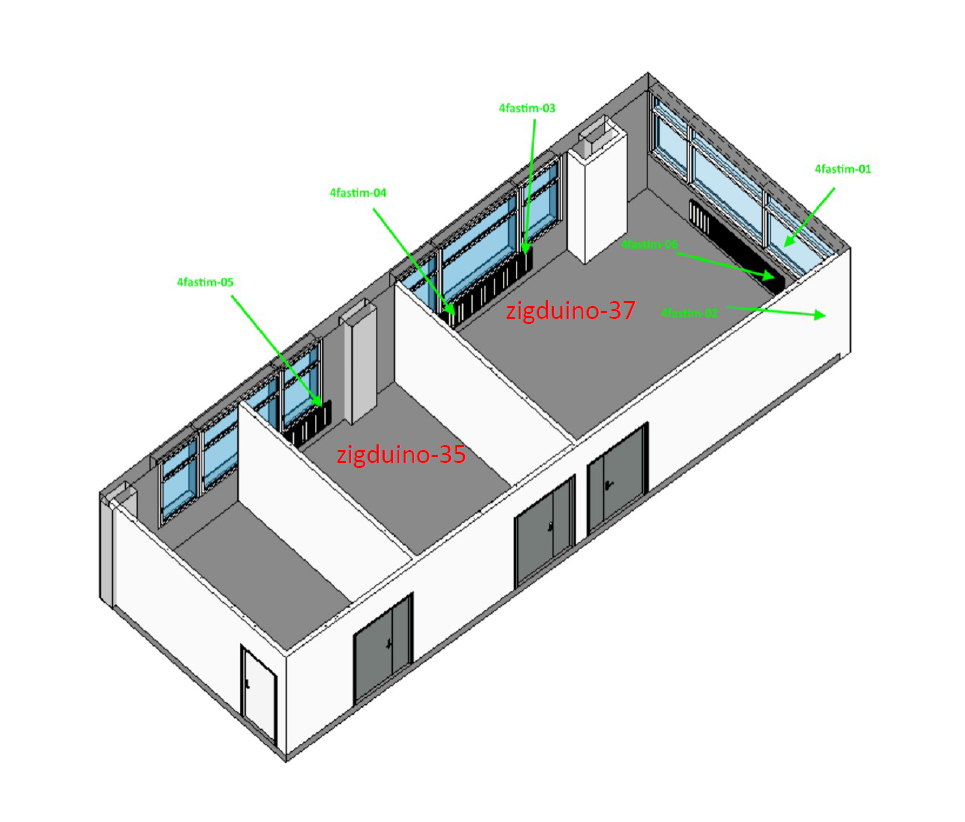
For our simulations, we are going to place ourselves in the 3 rooms considered, and use the temperature and humidity data obtained from the zigduino and 4fastsim sensors placed as in figure 1.

Note that we are actually doing our simulations in the 2 rooms of the 3 that contain the sensors.

However, as the 4fastsim sensors are placed directly next to the radiators, they present temperatures that can rise above \(47°C\) which is unfortunately less interesting for our simulations where we are working with an ambient room temperature. Thus, we will focus on the temperature and humidity data of the zigduino sensors. Furthermore, we will, as previously announced, consider 3 periods (cold, normal, warm) for our simulations, as well as the case of a female and a male patient.

The measurements for these 3 periods took place on February 18th (cold), April 23rd (normal) and July 21st (warm) of 2021. On these 3 days the data were always requested from 8am to 5pm.
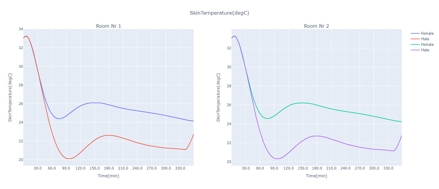
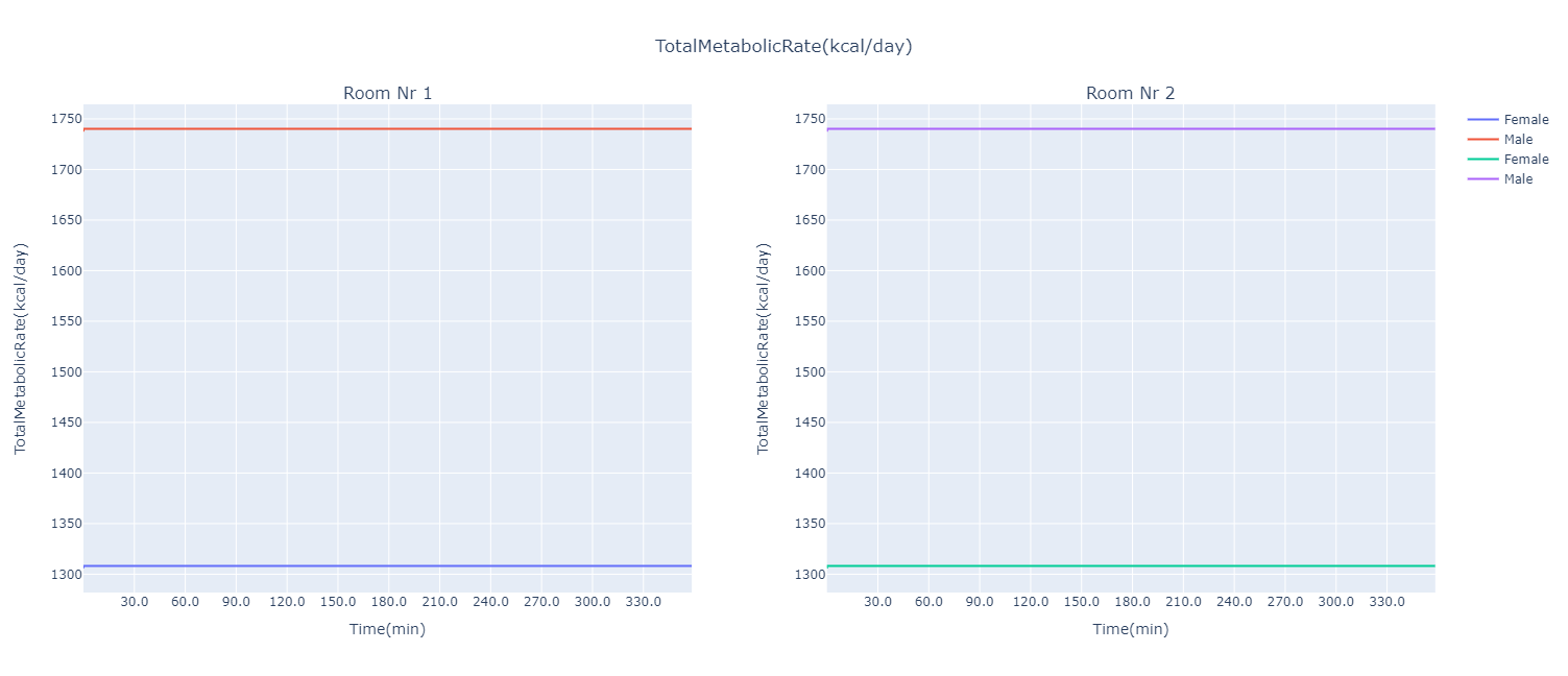
Moreover, we are especially interested in the output values of the skin temperature and the total metabolic rate.

However, it should be noted that Pulse did not run each time its simulations on these whole 9 hours, with one reason being that these simulations are really long as Pulse gives results for each \(0.02\; s\). Therefore, it should be noted that the simulations took about \(1\; h\; 25\; min\) for a specific room, gender and time period.

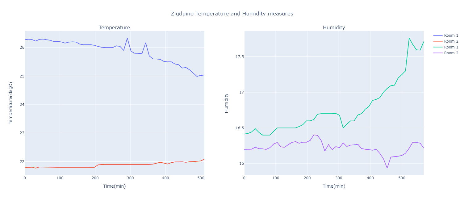
3.2.1. Cold (18.02.2021)

Figure 2. Temperature and Humidity

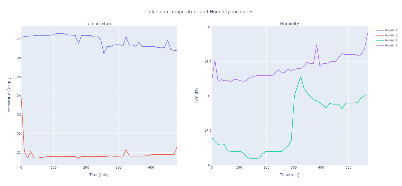
It can be seen that the temperatures are quite high for the period considered as cold. This is due to the use of radiators to heat the room. It can also be seen that there is a fairly clear difference between the two rooms in terms of temperature (up to \(6°C\)).
Regarding humidity, it can be seen that the values are very small. In fact, one could even say that these measured values are probably a little lower than those in reality. However, it can be said that the humidity in both rooms is very low.

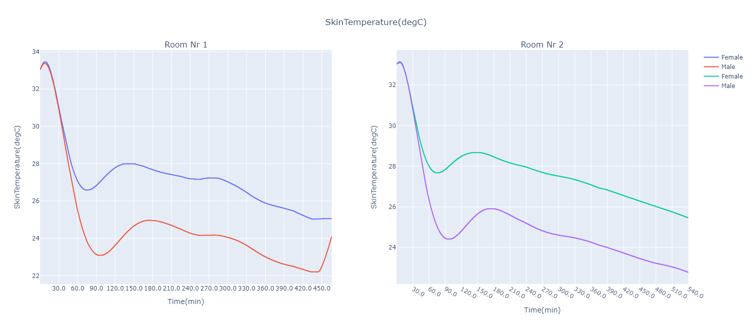
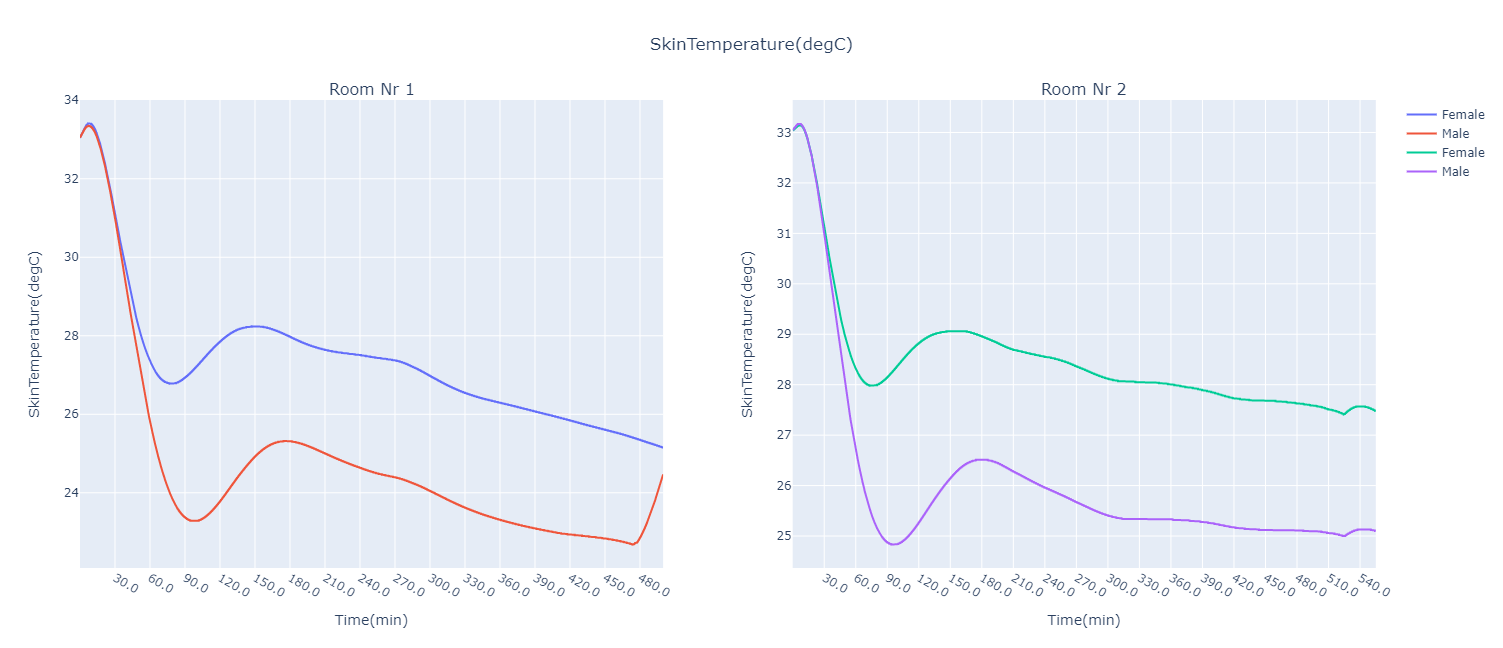
Figure 3. Skin Temperature for different rooms

It is observed that the skin temperature starts to drop only after a few minutes. After \(30\; min\), the curves of the two sexes start to differentiate with the skin temperature of the female being higher than that of the male. The two curves rebound after their local minimum obtained at \(75\; min\) and \(110\; min\). Then, the curves continue to fall. Finally, we observe a rise in the skin temperature of the male at the end around \(440\; min\).

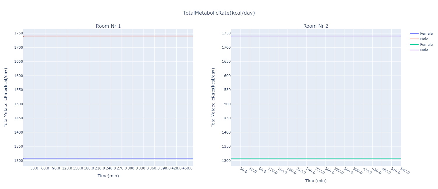
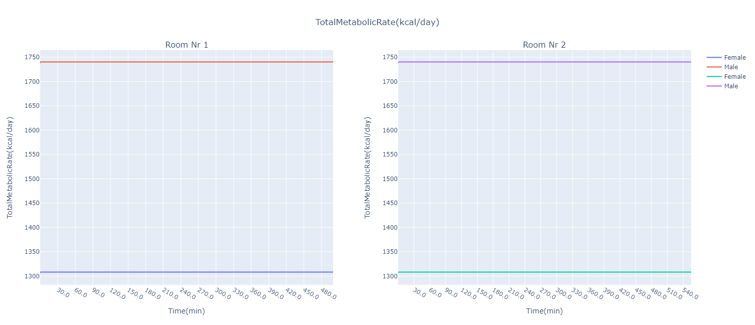
Figure 4. Total Metabolic Rate for different rooms

Concerning the total metabolic rate of both sexes, it can be seen that they are constant over time. It can be seen that the value of the male (\(\approx\; 1740\; kcal/day\)) is always higher than that of the female (\(\approx\; 1310\; kcal/day\)), regardless of the room.

3.2.2. Normal (23.04.2021)

Figure 5. Temperature and Humidity

It can be seen that the temperature of room 1 decreases over time, although there are two peaks at around \(290\; min\) and \(345\; min\). For room 2, the opposite is observed with a curve that increases over time.
The humidity is again quite low for both rooms. While there is little change in room 2, the curve for room 1 rises with more than \(1\%\) difference.

Figure 6. Skin Temperature for different rooms

The graphs obtained for room 1 are almost identical to those of the cold period, except that this time there is no slight increase in the curves around \(285\; min\). For room 2, the measured skin temperatures are slightly higher than those of the cold period, and drop less significantly once the \(180\; min\) is passed.

Figure 7. Total Metabolic Rate for different rooms

We see exactly the same results as in the previous case with exactly the same values.

3.2.3. Warm (21.07.2021)

Figure 8. Temperature and Humidity

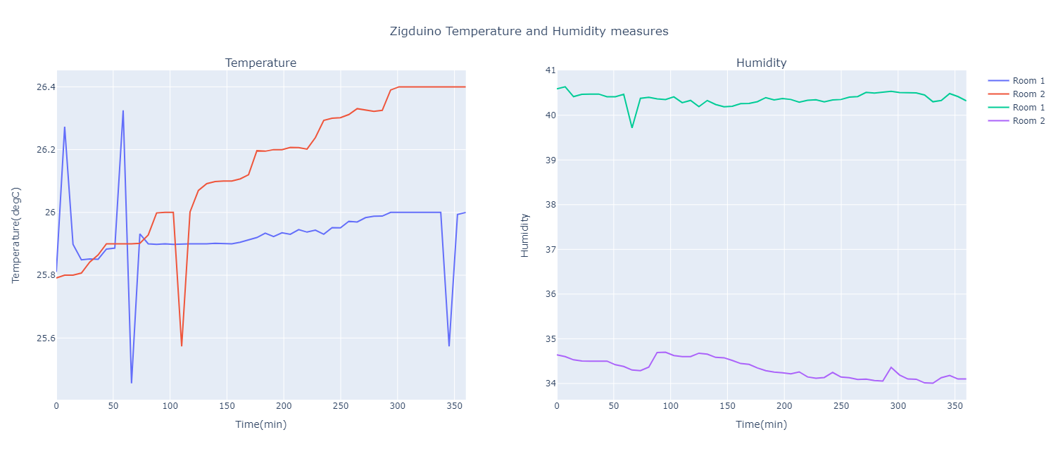
This time we get curves with more pronounced temperature changes. This may indeed be the exact temperatures of the rooms, or it may be slight inaccuracies of the sensors. In any case, both curves tend to increase.
In this period, which is considered to be warm, much higher humidity percentages can be observed than in the two previous cases. This time they are around \(40.5\%\) and \(34.5\%\) respectively.

Figure 9. Skin Temperature for different rooms

Firstly, it should be noted that the Pulse simulations only covered about \(358\; min\), which explains the slightly rightward shifting curves at first sight. However, the same curve shapes are again obtained as in the previous cases.

Figure 10. Total Metabolic Rate for different rooms

Finally, we find again the same graphs as for the other cases. It can be concluded that temperature and humidity do not really influence the values of the total metabolic rate.

References

[IB] IBat cases (2021, July 27). University building. Retrieved from cases.ibat.cemosis.fr/ibat.cases/0.1.0/cases/public_buildings/apiB.html.
[AV] Designing Buildings Wiki (2021, July 13). Indoor air velocity. Retrieved from designingbuildings.co.uk/wiki/Indoor_air_velocity.
[CR] Pulse (2021, July 13). Environment Methodology. Retrieved from pulse.kitware.com/_environment_methodology.html.
[EM] Optotherm (2021, July 2). Emissivity Values. Retrieved from optotherm.com/emiss-table.htm.
[RVOW] fatsecret (2021, July 14). Travail de Bureau. Retrieved from fatsecret.fr/fitness/travail-de-bureau.
[CL] ConvertLIVE (2021, July 14). Calories per hour to Watts. Retrieved from convertlive.com/u/convert/calories-per-hour/to/watts.
[PE] Pulse (2021, July 14). Energy Methodology. Retrieved from pulse.kitware.com/_energy_methodology.html.