Explanation of the method

Parareal method needs a decomposition of the time interval $[t_0,T$] into $P$ slices $[t_j,t_{j+1}$] with $j\in\{0,\dots,P-1\}$, where $P$ is the number of process units. As we want to parallelize the algorithm, each time slice is assigned to one process.

We denote by $F$ an integrator which is of high accuracy and $G$ which is of low accuracy. Also, $F$ will be very expensive in terms of calculation but very accurate, and $G$ will be very cheap but very imprecise. We denote by $\Delta t_F$ the time step and by $\Delta t_G$ the coarse time step.

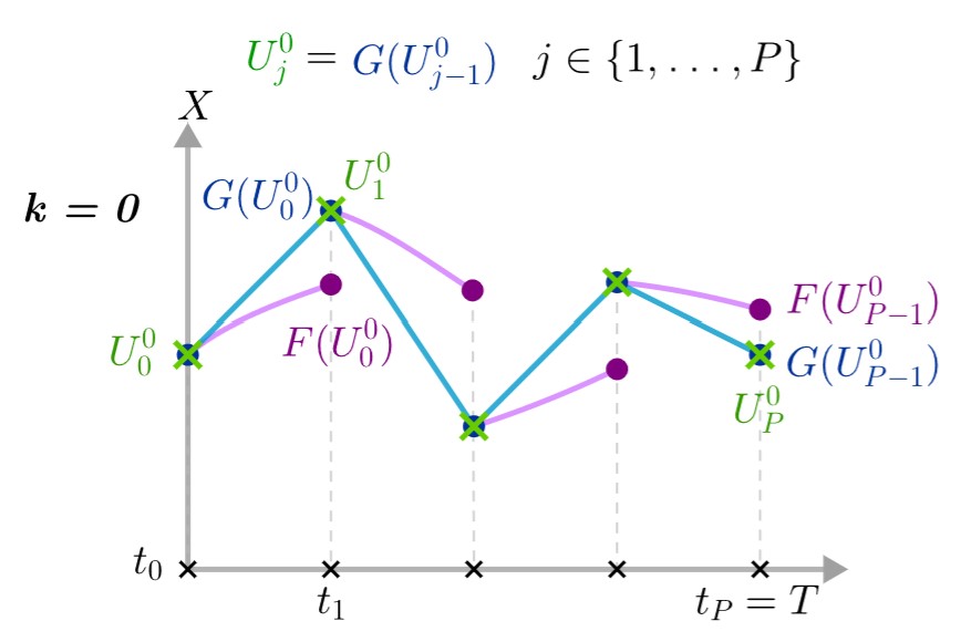
We denote by $U_j^k$, $j\in\{0,\dots,P\}$ the initial point at time $t_j$ and at iteration $k$. We also denote $F(U_{j-1}^k)$, $j\in\{1,\dots,P\}$ the result of the fine integrator between $t_{j-1}$ and $t_j$ which starts from the initial point $U_{j-1}^k$ at iteration $k$ and respectively $G(U_{j-1}^k)$, $j\in\{1,\dots,P\}$ the result of the coarse integrator between $t_{j-1}$ and $t_j$ which starts from the initial point $U_{j-1}^k$ at iteration $k$. Then, a series of steps is performed until the solution of the system converges.

At iteration $k=0$ :

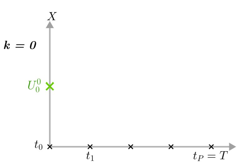
Step 1 : At iteration $k=0$, we have an initial point $U_0^0=X_0$.
Step 2 : We start by applying the function $G$ on all intervals $[t_j,t_{j+1}$] and we denote by $U_j^0=G(U_{j-1}^0)$ the values of $G$ at $t_j$.

This part of the method must be done sequentially because if we parallelize the task, the process $j$ should wait until the process $j-1$ has finished before starting.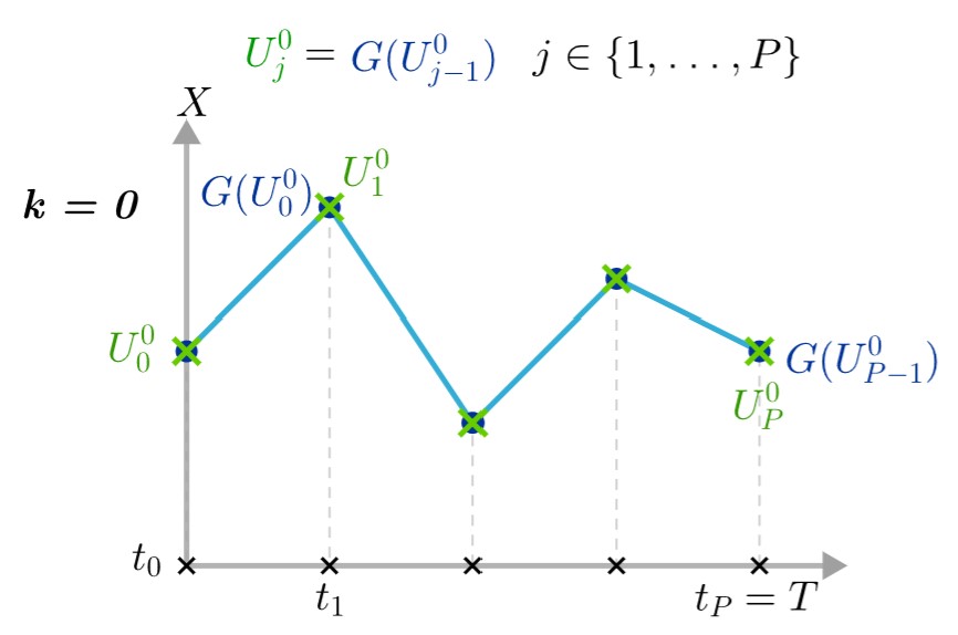
Step 3 : We can then calculate from each $U_j^0$ the fine solution between $t_j$ and $t_{j+1}$ : $F(U_j^0)$. This is an operation that must be parallelized.

At iteration $k=1$ :

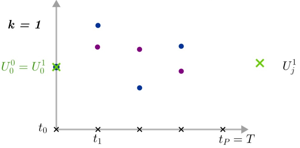
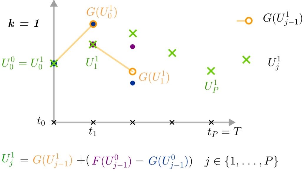
Step 4 : We can then continue to iteration $k=1$ where we need the values $G(U_j^0)$ and $F(U_j^0)$ calculated at the previous iteration ($k=0$).

We will also keep the initial point at time $t_0$ : $U_0^1=U_0^0$.
Step 5 : We can then calculate $G(U_0^1)$ which allows us to obtain the point $U_1^1$ by the following formula:

\[U_j^1=G(U_{j-1}^1)+(F(U_{j-1}^0)-G(U_{j-1}^0)).\]

due to the fact that $U_0^1=U_0^0$, we have $G(U_0^1)=G(U_0^0)$ and therefore $U_1^1=F(U_0^0)$.

We then compute in the same way the following $G(U_j^1)$ and the associated $U_{j+1}^1$ points. This step can be done sequentially for the same reason as in step 2.
Step 6 : We can then calculate from each $U_j^1$ the fine solution between $t_j$ and $t_{j+1}$ : $F(U_j^1)$. This is an operation that must be parallelized.

Note that due to $U_0^1=U_0^0$, we also have $F(U_0^1)=F(U_0^0)$.

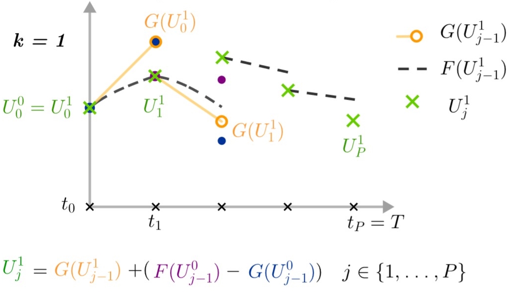
Then we repeat steps 3 to 6 until $U_j^k-U_j^{k-1}\rightarrow 0 \quad \forall j\in\{0,\dots,P-1\}$.

We have at iteration $k$:

\[U_j^k=G(U_{j-1}^k)+(F(U_{j-1}^{k-1})-G(U_{j-1}^{k-1}))\]